Rootfinding, Newton’s Method, and Dynamical Systems
Contents
Rootfinding, Newton’s Method, and Dynamical Systems#
In the Continued Fractions unit, we met with the sequence
which was generated by \(x_{n+1} = \frac12{\left(x_{n} + \frac{2}{x_n}\right)}\); in words, the average of the number and two divided by the number. This unit explores where that sequence came from, and its relationship to \(\sqrt{2}\).
A note to the Student/Reader#
This OER is beginning to take off. This unit is fairly short, but there are some nonstandard things in it.
We depend on your being able to take the derivative of a polynomial, or some other simple functions. We hope that you are becoming more comfortable with Python, and enjoy the activities from this unit.
A note to the Instructor#
Students can have quite a bit of fun with this. The notion of solving an equation approximately is quite familiar to many of them. Making the connections to the continued fraction unit, and to the Fibonacci unit, may make it even more interesting.
We try hard not to use the word “convergence”. It slips in from time to time, though. But we regard that as “stealing the thunder” from the calculus course, or the numerical analysis course. We also mention the very useful notion of continuation methods, also called homotopy methods (although that word gets used in different senses also).
Something that may be different for you as the instructor: we don’t look at the forward error of our approximation, that is \(|x_k - x^*|\) where \(x^*\) is the true (reference) root of the equation. Something that many students have trouble with is, if you know what \(x^*\) is, why are you approximating it? So instead we use backward error: if the residual is \(r_k = f(x_k)\) then we have found the exact solution of, not \(f(x) = 0\), but \(f(x) - r_k = 0\). This can make a great deal of sense in (say) an engineering context, and indeed we find that engineering students grasp the point straight away. But it is not really mathematics, because it depends on the context of the problem and one is left wondering if the \(r_k\) is small enough in that context (or is “physically meaningful”). One also worries about the impact of such changes in the problem on the answer, and this of course is the notion of sensitivity or conditioning. It’s also an excellent exercise in taking derivatives.
The most important question from the students for this section, and it’s a very natural one, is “how does one choose an initial estimate?” That of course leads to the next unit on fractals. Our friend David Jeffrey warns us against the phrase “initial guess” instead of “initial estimate”, by the way, and he’s right: we shouldn’t use it. It’s rare that someone actually just guesses to get an initial estimate.
Newton’s method and the square root of 2#
We’ll approach this algebraically, as Newton did. Consider the equation
Clearly the solutions to this equation are \(x = \sqrt{2}\) and \(x = -\sqrt{2}\). Our task, then, is to find approximations to the square root of \(2\). How shall we begin? We begin with an initial estimate for \(\sqrt{2}\). We choose the initial estimate \(x_0 = 1\).
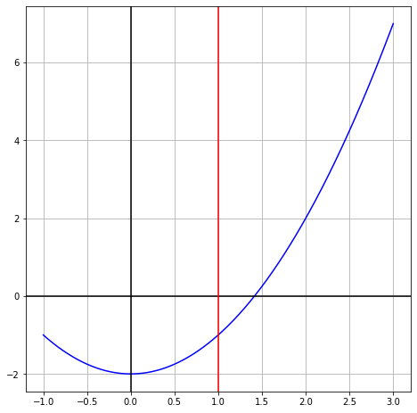
Let us now shift the origin by putting \(x = 1 + s\); so \(s = 0\) corresponds to our initial estimate \(x = 1\). This simply “centers the equation” at the (initial) estimate.
Now let us shift to a graphical view. We draw the vertical part of the new axis that we will shift to, in red. Notice that we use the labels and tickmarks from the old axis, in black.
import numpy as np
from matplotlib import pyplot as plt

fig = plt.figure(figsize=(6, 6))
ax = fig.add_axes([0,0,1,1])
n = 501
x = np.linspace(-1,3,n)
y = x*x-2;

plt.plot(x,y,'b')   # x^2-2 is in blue
ax.grid(True, which='both')
ax.axhline(y=0, color='k')
ax.axvline(x=0, color='k')
ax.axvline(x=1, color='r') # The new axis is in red
plt.show()
Then
we now make the surprising assumption that \(s\) is so small that we may ignore \(s^2\) in comparison to \(2s\). If it turned out that \(s = 10^{-6}\), then \(s^2 = 10^{-12}\), very much smaller than \(2s = 2\cdot10^{-6}\); so there are small numbers \(s\) for which this is true; but we don’t know that this is true, here. We just hope.
fig = plt.figure(figsize=(6, 6))
ax = fig.add_axes([0,0,1,1])
n = 501
s = np.linspace(-1,1,n)
y = -1+2*s+s*s;  # Newton would have written s^2 as s*s, too

plt.plot(s,y,'b')   # equation in blue again
ax.grid(True, which='both')
ax.axhline(y=0, color='r')
ax.axvline(x=0, color='r')
ax.axvline(x=1/2, color='k') # The new axis is in black
plt.show()
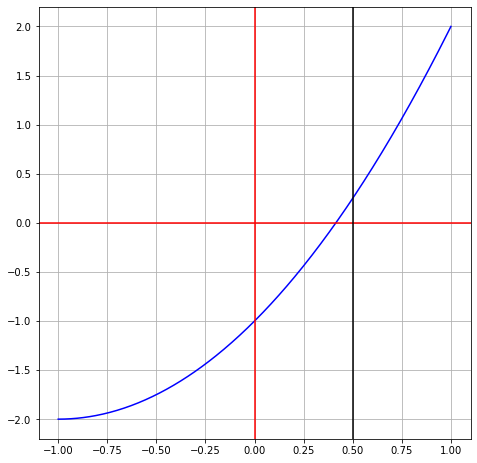
Then if \(s^2\) can be ignored, our equation becomes
or \(s = \frac{1}{2}\). This means \(x = 1 + s = 1 + \frac{1}{2} = \frac{3}{2}\).
We therefore have a new estimate for the root. We could call it \(x_1\) if we liked, and \(x_1 = \frac32\).
We now repeat the process: shift the origin to \(\frac{3}{2}\), not \(1\): put now
which is equivalent to \(s = 1/2 + t\), so
fig = plt.figure(figsize=(6, 6))
ax = fig.add_axes([0,0,1,1])
n = 501
t = np.linspace(-0.2,0.2,n)
y = 1/4+3*t+t*t;  # Newton would have written t^2 as t*t, too

plt.plot(t,y,'b')   # equation in blue again
ax.grid(True, which='both')
ax.axhline(y=0, color='k')
ax.axvline(x=0, color='k')
ax.axvline(x=-1/12, color='r') # The new axis will be red again
plt.show()
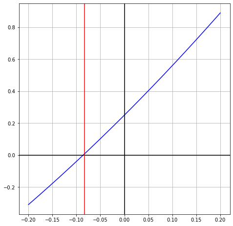
This gives \(3t + t^2 + \frac{1}{4} = 0\) and again we ignore \(t^2\) and hope it’s smaller than \(3t\). This gives
or \(t = -\frac{1}{12} \approx -0.08333\). This means \(x = \frac{3}{2} - \frac{1}{12}\) or \(x = \frac{17}{12}\). Now we see the process.
Again, shift the origin: \(x = \frac{17}{12} + u\). Now
Ignoring \(u^2\),
or
Thus,
As we saw in the Continued Fractions unit, these are the exact square roots of numbers ever more close to 2. For instance,
Euler again#
It was Euler who took Newton’s “shift the origin” strategy and made a general method—which we call Newton’s method—out of it. In modern notation, Euler considered solving \(f(x) = 0\) for a differentiable function \(f(x)\), and used the tangent line approximation near an initial approximation \(x_0\): if \(x = x_0 + s\) then, using \(f'(x_0)\) to denote the slope at \(x_0\), \(0 = f(x) = f(x_0 + s) \approx f(x_0) + f'(x_0)s\) ignoring terms of order \(s^2\) or higher. Then
so
The fundamental idea of Newton’s method is that, if it worked once, we can do it again: pass the parcel! Put
and keep going, until \(f(x_k)\) is so small that you’re happy to stop.
Notice that each \(x_k\) solves
not \(f(x) = 0\). But if \(f(x_k)\) is really small, you’ve solved “almost as good” an equation, like finding \(\sqrt{2 + \frac{1}{408^2}}\) instead of \(\sqrt{2}\). So where did \(\frac12{\left(x_n + \frac{2}{x_n}\right)}\) come from?
because if \(f(x) = x^2 - 2\), \(f'(x) = 2x - 0 = 2x\). Therefore,
as claimed. (For more complicated functions one shouldn’t simplify, because the construct “approximation” plus (or minus) “small change” is more numerically stable, usually. But for \(x^2 - a\), it’s okay.)
Executing this process in decimals, using a calculator (our handy HP48G+ again), with \(x_0 = 1\), we get
Now \(\sqrt{2} = 1.41421356237\) on this calculator. We see (approximately) 1, 2, 5 then 10 correct digits. The convergence behaviour is clearer in the continued fraction representation:
with 0, 1, 3, 7, 15 twos in the fraction part: each time doubling the previous plus 1, giving \(2^0 - 1\), \(2^1 - 1\), \(2^2 - 1\), \(2^3 - 1\), \(2^4 - 1\) correct entries. This “almost doubling the number of correct digits with each iteration” is quite characteristic of Newton’s method.
Newton’s Method#
In the Continued Fractions unit, we saw Newton’s method to extract square roots: \(x_{n+1} = (x_n + a/x_n)/2\). That is, we simply took the average of our previous approximation with the result of dividing our approximation into what we wanted to extract the square root of. We saw rapid convergence, in that the number of correct entries in the continued fraction for \(\sqrt{a}\) roughly doubled with each iteration. This simple iteration comes from a more general technique for finding zeros of nonlinear equations, such as \(f(x) = x^5 + 3x + 2 = 0\). As we saw above, for general \(f(x)\), Newton’s method is
where the notation \(f'(x_n)\) means the derivative of \(f(x)\) evaluated at \(x=x_n\). In the special case \(f(x) = x^2-a\), whose roots are \(\pm \sqrt{a}\), the general Newton iteration above reduces to the simple formula we used before, because \(f'(x) = 2x\).
Derivatives#
We’re not assuming that you know so much calculus that you can take derivatives of general functions, although if you do, great. We could show a Python method to get the computer to do it, and we might (or we might leave it for the Activities; it’s kind of fun). But we do assume that you know that derivatives of polynomials are easy: for instance, if \(f(x) = x^3\) then \(f'(x) = 3x^2\), and similarly if \(f(x) = x^n\) for some integer \(n\) then \(f'(x) = n x^{n-1}\) (which holds true even if \(n\) is zero or a negative integer—or, for that matter, if \(n\) is any constant). Then by the linearity of the derivative, we can compute the derivative of a polynomial expressed in the monomial basis. For instance, if \(f(x) = x^5 + 3x + 2\) then \(f'(x) = 5x^4 + 3\). It turns out that the Python implementation of polynomials knows how to do this as well (technically, polynomials know how to differentiate themselves), as we will see. For this example we can use this known derivative in the Newton formula to get the iteration
Rootfinding Activity 1
Write Newton’s method iterations for the following functions, and estimate the desired root(s).
\(f(x) = x^2 - 3\) with \(x_0 = 1\)
\(f(x) = x^3 - 2\) with \(x_0 = 1\)
Newton’s original example, \(f(x) = x^3 - 2x - 5 = 0\). Since \(f(0) = -5\), \(f(1) = -6\), \(f(2) = -1\), and \(f(3) = 16\), we see there is a root between \(x=2\) and \(x=3\). Use that knowledge to choose your initial estimate. [What happened when we did this]
Rootfinding Activity 1
The Railway Pranksters Problem
Late one night, some pranksters weld a \(2\)cm piece of steel into a train track \(2\)km long, sealing the gaps meant to allow for heat expansion. In the morning as the temperature rises, the train track expands and bows up into a perfectly circular arc. How high is the arc in the middle? [How we found the height]
A more serious application#
where the mean anomaly \(M = n(t-t_0)\) where \(t\) is time, \(t_0\) is the starting time, \(n = 2\pi/T\) is the sweep speed for a circular orbit with period \(T\), and the eccentricity \(e\) of the (elliptical) orbit are all known, and one wants to compute the eccentric anomaly \(E\) by solving that nonlinear equation for \(E\). Since we typically want to do this for a succession of times \(t\), initial estimates are usually handy to the purpose (just use the \(E\) from the previous instant of time), and typically only one Newton correction is needed.
T = 1 # Period of one Jupiter year, say (equal to 11.8618 earth years)
n = 2*np.pi/T
# At t=t_0, which we may as well take to be zero, M=0 and so E = 0 as well.
nsamples = 12 # Let's take 13 sample positions including 0.
e = 0.0487 # Jupiter has a slightly eccentric orbit; not really visible to the eye here
E = [0.0]
f = lambda ee: ee-e*np.sin(ee)-M
df = lambda ee: 1 - e*np.cos(ee)
newtonmax = 5
for k in range(nsamples):
    M = n*(k+1)/nsamples # measuring time in Jupiter years
    EE = E[k]
    newtoniters = 0
    for j in range(newtonmax):
        residual = f(EE);
        if abs(residual) <= 1.0e-12:  # A hard-coded "timeout" which seems reasonable
            break                     # A new statement: stop the loop if this happens
        EE = EE - residual/df(EE)
    E.append(EE)
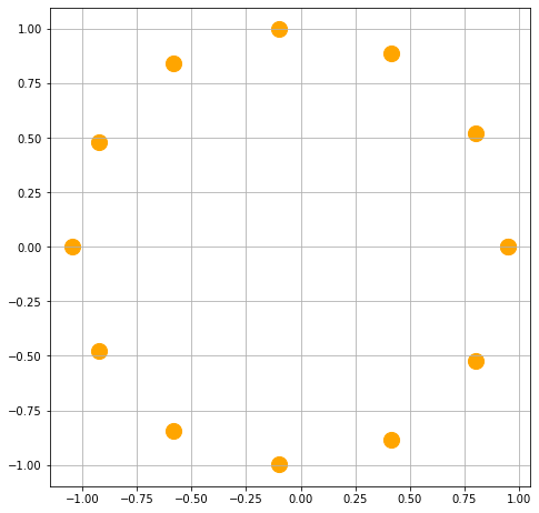
That loop computes a bunch of values of the eccentric anomaly E for an equally-spaced collection of M values. The next block plots the coordinates of the orbiting body given the value of E. We represent the body by a circle of size s=200 and colour it orange.
x = [np.cos(ee)-e for ee in E]
y = [np.sqrt(1-e*e)*np.sin(ee) for ee in E]
fig = plt.figure(figsize=(6, 6))
ax = fig.add_axes([0,0,1,1])
plt.scatter(x,y,s=200,color='orange')
ax.set_aspect('equal')
ax.grid(True, which='both')
plt.show()
A useful interpretation#
When we were looking at square roots, we noticed that each iteration (say \(17/12\)) could be considered the exact square root of something near to what we wanted to extract the root of; this kind of interpretation is possible for general functions as well. Each iterate \(x_n\), when we are trying to solve \(f(x) = 0\), can be considered to be the exact zero of \(g(x) = f(x)-r_n\), where \(r_n = f(x_n)\) is the so-called residual. The equation is so simple that it’s slippery: \(x_n\) solves \(f(x) - f(x_n) = 0\). Of course it does. No matter what you put in for \(x_n\), so long as \(f(x)\) was defined there, you would have a zero. The key of course is the question of whether or not the residual is small enough to ignore. There are two issues with that idea.
The function \(f(x)\) might be sensitive to changes (think of \(f(x) = (x-\pi)^2\), for instance; adding just a bit to it makes both roots complex, and the change is quite sudden).
The change might not make sense in the physical/chemical/biological context in which \(f(x)\) arose.
This second question is not mathematical in nature: it depends on the context of the problem. Nevertheless, as we saw for the square roots, this is often a very useful look at our computations.
To answer the question of sensitivity, we need calculus, and the general notion of derivative:
\(f(x)+s = 0\) makes some kind of change to the zero of \(f(x)=0\), say \(x=r\). If the new root is \(x=r+t\) where \(t\) is tiny (just like \(s\) is small) then calculus says \(0 = f(r+t) + s = f(r)+f'(r)t+s + O(t^2)\) where we have used the tangent-line approximation (which is, in fact, where Newton iteration comes from). Solving for this we have that \(t = -s/f'(r)\), because of course \(f(r)=0\).
This is nothing more (or less!) than the calculus derivation of Newton’s method, but that’s not what we are using it for here. We are using it to estimate the sensitivity of the root to changes in the function. We see that if \(f'(r)\) is small, then \(t\) will be much larger than \(s\); in this case we say that the zero of \(f(x)\) is sensitive. If \(f'(r)=0\) we are kind of out of luck with Newton’s method, as it is; it needs to be fixed up.
Things that can go wrong#
Newton’s method is a workhorse of science, there’s no question. There are multidimensional versions, approximate versions, faster versions, slower versions, applications to just about everything, especially optimization. But it is not a perfect method. Solving nonlinear equations is hard. Here are some kinds of things that can go wrong.
The method can give a sequence that tends to the wrong root. If there’s more than one root, then this can happen.
The method can divide by zero (if you happen to hit a place where the derivative is zero). Even just with \(f(x)=x^2-2\) this can happen if you choose your initial estimate as \(x_0 = 0\). (See if you can either find other \(x_0\) that would lead to zero, or else prove it couldn’t happen for this function).
If the derivative is small but not zero the iteration can be very, very slow. This is related to the sensitivity issue.
You might get caught in a cycle (see the animated GIF in the online version). That is, like with the game of pass the parcel with the Gauss map, we may eventually hit the initial point we started with.
The iteration may wander a long way before seeming to suddenly tend to a root.
The iteration may go off to infinity.
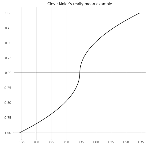
Let’s take Cleve Moler’s “perverse example”, from section 4.3 of Numerical Computing with Matlab, namely
We will draw this in the next cell, for some harmless \(r\). This peculiar function was chosen so that every initial estimate (that wasn’t exactly right, i.e. \(x=r\)) would create a two-cycle: pretty mean.
Let’s check. The derivative is
So the Newton iteration is, if \(x_n > r\),
which can be rewritten to be \(x_{n+1}-r = r -x_n\), so the distance to \(r\) is exactly the same but now we are on the other side. If instead \(x_n < r\),
which again says \(x_{n+1}-r = r -x_n\).
In particular, take \(x_0 = 0\). Then \(x_1 = 2r\). Then \(x_2 = 0\) again.
Obviously this example was contrived to show peculiar behaviour; but these things really can happen.
r = 0.73  # Some more or less random number
n = 501
x = np.linspace(-1+r,1+r,n)
y = np.sign(x-r)*np.sqrt(np.abs(x-r))

fig = plt.figure(figsize=(6, 6))
ax = fig.add_axes([0,0,1,1])

plt.plot(x,y,'k')
ax.grid(True, which='both')
ax.axhline(y=0, color='k')
ax.axvline(x=0, color='k')
plt.title("Cleve Moler's really mean example")
plt.show()
Rootfinding Activity 3
Take a few moments and write down some questions about Newton’s method or rootfinding in general. Do not worry about answers, just now. [Some of the questions we thought of]
A Really Useful trick to find initial estimates#
One of our “generic good questions” was “can you find an easier question to solve?” and “does answering that easier question help you to to solve this one?” This gives an amazing method, called continuation or homotopy continuation for solving many equations, such as polynomial equations. The trick is easily stated. Suppose you want to solve \(H(x) = 0\) (H for “Hard”) and you have no idea where the roots are. You might instead be able to solve \(E(x) = 0\), a similar equation but one you know the roots of already (E for “Easy”, of course). Then consider blending them: \(F(x,t) = (1-t)E(x) + tH(x)\) for some parameter \(t\), which we take to be a real number between \(0\) and \(1\).
You start by solving the Easy problem, at \(t=0\), because \(F(x,0) = E(x)\). Then increase \(t\) a little bit, say to \(t=0.1\); use the roots of \(E(x)\) as your initial estimate of the roots of \(F(x,0.1) = 0.9E(x) + 0.1H(x)\). If it works, great; increase \(t\) again, and use those recently-computed roots of \(F(x,0.1)\) as the initial estimates for (say) \(F(x,0.2)\). Continue on until either the method breaks down (it can, the root paths can cross, which is annoying, or go off to infinity, which is worse) or you reach the end.
As an example, suppose you want to solve \(h(x) = x e^x - 2.0 = 0\). (This isn’t a very hard problem at all, but it’s a nice example). If we were trying to solve \(e(x) = e^x - 2.0 = 0\), then we already know the answer: \(x=\ln(2.0) = 0.69314718056\ldots\). So \(f(x,t) = (1-t)(e^x - 2) + t(xe^x -2) = (1-t+tx)e^x - 2 = (1+t(x-1))e^x - 2\). Newton’s method for this is straightforward (this is the first non-polynomial function we’ve used, but we bet that you know that the derivative of \(e^x\) is \(e^x\), and that you know the product rule as well). So our iteration is (for a fixed \(t\))
nt = 10
newtonmax = 3
t = np.linspace(0,1,nt)
x = np.zeros(nt+1)
x[0] = np.log(2.0) # Like all snobs, Python insists on log rather than ln
for k in range(1,nt):
    xi = x[k-1]
    for i in range(newtonmax):
        y = np.exp(xi)
        ft = (1+t[k]*(xi-1))*y-2;
        dft = (1-t[k] + t[k]*(xi+1))*y
        xi = xi - ft/dft
    x[k] = xi

print( 'The solution is {} and the residual is {}'.format(xi, xi*np.exp(xi)-2.0) )
The solution is 0.8526055020137254 and the residual is -2.220446049250313e-16
from scipy import special
reference = special.lambertw(2.0)
print("The reference value is {}".format(reference))
The reference value is (0.8526055020137254+0j)
For some unknown reason (probably just to make the programmer’s life a little easier), the SciPy value of the Lambert \(W\) function is of type complex, even though it has zero imaginary part. But the real part is the same as what we had computed by Newton’s method. You can learn more about the Lambert W function here or at the Wikipedia link.
The problem with multiple roots#
Newton’s iteration divides by \(f'(x_n)\), and if the root \(r\) we are trying to find happens to be a multiple root, that is, both \(f(r) = 0\) and \(f'(r)=0\), then the \(f'(x_n)\) we are dividing by will get smaller and smaller the closer we get to \(r\). This slows Newton iteration to a crawl. Consider \(f(x) = W(x^3)\) where \(W(s)\) is the Lambert W function. Then since \(W(0)=0\) we have \(f'(x) = 3x^2 W'(x^3)\) so \(f'(0)=0\) as well. Let’s look at how this slows us down. Notice that \(W(s)\) is itself defined to be the root of the equation \(y\exp(y)-s = 0\), and it itself is usually evaluated by an iterative method (in Maple, Halley’s method, which we will talk about in the next unit, is used because the derivatives are cheap). But let’s just let Python evaluate it for us here. We can evaluate \(W'(x)\) by implicit differentiation: \(W(x)\exp W(x) = x\) so \(W'(x)\exp W(x) + W(x) W'(x) \exp W(x) = 1\) and therefore \(W'(x) = 1/(\exp W(x)(1+ W(x)))\).
Counting Brackets
One of the more obnoxious things about programming is making sure your brackets [] match, your parens () match, and your braces {} match. Python doesn’t use angle brackets <> but does use < and > in arithmetic comparisons, which is natural enough.
But lists use brackets [] and tuples use parens (), and these have to occur in left-right pairs. All that is ok and not usually a problem. Where most of the trouble with “fences” (as all these are called) comes from expressions, especially nested expressions. Making sure your parens match up the right way (in the way that you intended) is really a pain. Eventually you get used to it, so much so that mismatched fences can be irritating to see. But in the beginning it’s hard. The only piece of advice we have is to be neat about it, and use whitespace where appropriate.
f = lambda x: special.lambertw( x**3 )
df = lambda x: 3*x**2/( np.exp(f(x))*(1+ f(x)) )
SirIsaac = lambda x: x - f(x)/df(x)
hex = [0.1] # We pretend that we don't know the root is 0
n = 10
for k in range(n):
    nxt = SirIsaac( hex[k] )
    hex.append( nxt )
print( hex )
[0.1, (0.06663336661675538+0j), (0.04441567513800068+0j), (0.029609152955240525+0j), (0.019739179108047566+0j), (0.013159402133893338+0j), (0.008772924760017679+0j), (0.005848614532183305+0j), (0.0038990759647654777+0j), (0.0025993838994686808+0j), (0.001732922584427687+0j)]
We can see that the iterates are decreasing but the turtle imitation is absurd.
There is an almost useless trick to speed this up. If we “just happen to know” the multiplicity \(\mu\) of the root, then we can speed things up. Here the multiplicity is \(\mu=3\). Then we can modify Newton’s iteration to speed it up, like so:
Let’s try it out.
mu = 3
ModSirIsaac = lambda x: x - mu*f(x)/df(x)
n = 3
hex = [0.2]
for k in range(n):
    nxt = ModSirIsaac( hex[k] )
    hex.append(nxt)
print( hex )
[0.2, (-0.0015873514490433727+0j), (-6.348810149478523e-12+0j), (8.077935669463161e-28+0j)]
So, it does work; instead of hardly getting anywhere in ten iterations, it got the root in three. NB: The first time we tried this, we had a bug in our derivative and the iterates did not approach zero with the theoretical speed: so we deduced that there must have been a bug in the derivative, and indeed there was.
But this trick is (as we said) almost useless; because if we don’t know the root, how do we know its multiplicity?
What happens if we get the derivative wrong?#
Let’s suppose that we get the derivative wrong—maybe deliberately, to save some computation, and we only use the original estimate \(f'(x_0)\). This can be useful in some circumstances. In this case, we don’t get such rapid approach to the zero, but we can get the iterates to approach the root, if not very fast. Let’s try. Take \(f(x) = x^2-2\), and our initial estimate \(x_0 = 1\) so \(f'(x_0) = 2\). This “approximate Newton” iteration then becomes
or \(x_{n+1} = x_n - (x_n^2-2)/2\).
n = 10
hex = [1.0]
f = lambda x: x*x-2
df = 2
quasi = lambda x: x - f(x)/df;
for k in range(n):
    nxt = quasi( hex[k] )
    hex.append(nxt)
print( hex )
[1.0, 1.5, 1.375, 1.4296875, 1.407684326171875, 1.4168967450968921, 1.4130985519638084, 1.4146747931827024, 1.4140224079494415, 1.4142927228578732, 1.4141807698935047]
We see that the iterates are getting closer to the root, but quite slowly.
To be honest, this happens more often when someone codes the derivative incorrectly than it does by deliberate choice to save the effort of computing the derivative. It has to be one ridiculously costly derivative before this slow approach is considered worthwhile (it looks like we get about one more digit of accuracy after two iterations).
What if there is more than one root?#
A polynomial of degree \(n\) has \(n\) roots (some or all of which may be complex, and some of which may be multiple). It turns out to be important in practice to solve polynomial equations. John McNamee wrote a bibliography in the late nineties that had about ten thousand entries in it—that is, the bibliography listed ten thousand published works on methods for the solution of polynomials. It was later published as a book, but would be best as a computer resource. Unfortunately, we can’t find this online anywhere now, which is a great pity. But in any case ten thousand papers is a bit too much to expect anyone to digest. So we will content ourselves with a short discussion.
First, Newton’s method is not very satisfactory for solving polynomials. It only finds one root at a time; you need to supply an initial estimate; and then you need to “deflate” each root as you find it, so you don’t find it again by accident. This turns out to introduce numerical instability (sometimes). This all can be done but it’s not so simple. We will see better methods in the Mandelbrot unit.
But we really don’t have to do anything: we can use Maple’s fsolve, which is robust and fast enough for most purposes. In Python, we can use the similarly-named routine fsolve from SciPy, if we only want one root: there are other facilities in NumPy for polynomial rootfinding, which we will meet in a later unit.
We do point out that the “World Champion” polynomial solver is a program called MPSolve, written by Dario Bini and Leonardo Robol. It is freely available at this GitHub link. The paper describing it is here.
from scipy.optimize import fsolve
f = lambda x: x**2+x*np.exp(x)-2
oneroot = fsolve( f, 0.5 )
print( oneroot, oneroot**2 + oneroot*np.exp(oneroot)-2 )
[0.72048399] [-2.44249065e-15]
Complex initial approximations, fractal boundaries, Julia sets, and chaos#
Using Newton’s method to extract square roots (when you have a calculator, or Google) is like growing your own wheat, grinding it to flour by hand, and then baking bread, when you live a block away from a good bakery. It’s kind of fun, but faster to do it the modern way. But even for cube roots, the story gets more interesting when complex numbers enter the picture.
Consider finding all \(z\) with
The results are \(z = 2\), \(z = 2\cdot e^{\frac{i\cdot2\pi}{3}}\), and \(z = 2\cdot e^{\frac{-i2\pi}{3}}\).
See our Appendix on complex numbers.
Now, you are ready to look at the next unit, where we will pursue what happens with complex initial estimates.
A look back at the programming constructs used in this unit#
We are assuming that you did not start with this unit. So, in addition to the things you saw in the previous unit(s), we mentioned new plotting features such as gridlines and other decorations. We saw the break statement for stopping a loop when a computed event happened (which couldn’t have been predicted ahead of time). We introduced linspace from numpy which is a very useful construct to get a vector of values equally spaced across an interval. The name is taken from the Matlab command of the same name; it’s not an intuitive name, but one gets used to it. We introduced lambda functions, which are good for one-line programs or even anonymous programs. The name comes from a philosophical approach to computing by Alonzo Church that compares with Turing machines. But for us it’s just syntax.
We didn’t comment on the “timeout” of the break statement. That loop quits if the absolute value of the residual is smaller than \(10^{-12}\). Why that number? And why was it hard-coded into the program? Why not \(10^{-11}\) or \(10^{-13}\)? There is no good answer to that. The precision is more than enough to produce a good graph, in this case. It’s better to use a named variable, say MINIMUM_RESIDUAL and set that in a visible spot at the beginning of the code, for large programs, in case it needs to be changed later after experience shows that the specific number chosen wasn’t, after all, a good idea. For this small demonstration program, there was not much harm (except possibly to your programming habits, because this is really a bad example to follow).
We saw the first use of colour in plots. We saw the first “special” function, namely Lambert \(W\). This is implemented in scipy. We saw complex numbers, and the optimize subpackage, and the solver fsolve.
More Activities#
Rootfinding Activity 4
Sometimes Newton iteration is “too expensive”; a cheaper alternative is the so-called secant iteration, which goes as follows: \(z_{n+1} = z_n - f(z_n)(z_{n}-z_{n-1})/(f(z_n) - f(z_{n-1}))\). You need not one, but two initial approximations for this. Put \(f(z) = z^2-2\) and start with the two initial approximations \(z_0 = 1\), \(z_1 = 3/2\). Carry out several steps of this (in exact arithmetic is better). Convert each rational \(z_n\) to continued fraction form. Discuss what you find. [What happened when we did this]
Rootfinding Activity 5
Try Newton and secant iteration on some functions of your own choosing. You should see that Newton iteration usually takes fewer iterations to converge, but since it needs a derivative evaluation while the secant method does not, each iteration is “cheaper” in terms of computational cost (if \(f(z)\) is at all expensive to evaluate, \(f'(z)\) usually is too; there are exceptions, of course). The consensus seems to be that the secant method is a bit more practical; but in some sense it is just a variation on Newton’s method. [What happened when we did this]
Rootfinding Activity 6
Both the Newton iteration and the secant iteration applied to \(f(z) = z^2-a^2\) can be solved analytically by the transformation \(z = a\coth \theta\). Hyperbolic functions The iteration \(z_{n+1} = (z_n + a^2/z_n)/2\) becomes (you can check this) \(\coth \theta_{n+1} = \cosh 2\theta_n/\sinh 2\theta_n = \coth 2\theta_n\), and so we may take \(\theta_{n+1} = 2\theta_n\). This can be solved to get \(\theta_n = 2^n\theta_0\) and so we have an analytical formula for each \(z_n = a \coth( 2^n \theta_0 )\). Try this on \(a^2=2\); you should find that \(\theta_0 = \mathrm{invcoth}(1/\sqrt{2})\). By “invcoth” we mean the functional inverse of coth, i.e.: \(\coth\theta_0 = 1/\sqrt{2}\). It may surprise you that that number is complex. Nevertheless, you will find that all subsequent iterates are real, and \(\coth 2^n\theta_0\) goes to \(1\) very quickly. NB This was inadvertently difficult. Neither numpy nor scipy has an invcoth (or arccoth) function. The Digital Library of Mathematical Functions says (equation 4.37.6) that arccoth(z) = arctanh(1/z). Indeed we had to go to Maple to find out that invcoth\((1/\sqrt{2}) = \ln(1+\sqrt{2}) - i\pi/2\). [What happened when we did this]
Rootfinding Activity 7
Try the above with \(a^2=-1\). NB the initial estimate \(z_0 = 1\) fails! Try \(z_0 = e = \exp(1) = 2.71828...\) instead. For this, the \(\theta_0 = 1j\arctan(e^{-1})\). Then you might enjoy reading Gil Strang’s lovely article A Chaotic Search for \(i\). [What happened when we did this]
Rootfinding Activity 8
Try to solve the secant iteration for \(z^2-a^2\) analytically. You should eventually find a connection to Fibonacci numbers. [What happened when we did this]
Rootfinding Activity 9
People keep inventing new rootfinding iterations. Usually they are reinventions of methods that others have invented before, such as so-called Schroeder iteration and Householder iteration. One step along the way is the method known as Halley iteration, which looks like this:
which, as you can see, also involves the second derivative of \(f\). When it works, it works quickly, typically converging in fewer iterations than Newton (although, typically, each step is more expensive computationally). Try the method out on some examples. It may help you to reuse your code (or Maple’s code) if you are told that Newton iteration on \(F(z) = f(z)/\sqrt{f'(z)}\) turns out to be identical to Halley iteration on \(f(z)\). NB: this trick helps you to “re-use” code, but it doesn’t generate a particularly efficient iteration. In particular, the square roots muck up the formula for the derivatives, and simplification beforehand makes a big difference to program speed. So if you want speed, you should program Halley’s method directly. [What happened when we did this]
Rootfinding Activity 10
Try to solve Halley’s iteration for \(x^2-a\) analytically. Then you might enjoy reading Revisiting Gilbert Strang’s “A Chaotic Search for i” by Ao Li and Rob Corless; Ao was a (graduate) student in the first iteration of this course at Western, and she solved—in class!—what was then an open problem (this problem!). [What happened when we did this]
Rootfinding Activity 11
Let’s revisit Activity 6. It turns out that we don’t need to use hyperbolic functions. In the OEIS when searching for the numerators of our original sequence \(1\), \(3/2\), \(17/12\) and so on, and also in the paper What Newton Might Have Known, we find the formulas \(x_n = r_n/s_n\) where
Verify that this formula gives the same answers (when \(a=2\)) as the formula in question 4. Try to generalize this formula for other integers \(a\). Discuss the growth of \(r_n\) and \(s_n\): it is termed doubly exponential. Show that the error \(x_n - \sqrt2\) goes to zero like \(1/(3+2\sqrt2)^{2^n}\). How many iterations would you need to get ten thousand digits of accuracy? Do you need to calculate the \((1-\sqrt2)^{2^n}\) part? [Where you can find more discussion]
Rootfinding Activity 12
Do any of the other results of Revisiting Gilbert Strang’s “A Chaotic Search for i” on secant iteration, Halley’s iteration, Householder iteration, and so on, translate to a form like that of Activity 11? (We have not tried this ourselves yet). [Some thoughts]
Rootfinding Activity 13
Solve the Schroeder iteration problem of the paper Revisiting Gilbert Strang’s “A Chaotic Search for i”. This iteration generates the image of the “infinite number of infinity symbols” used in the Preamble, by the way. We don’t know how to solve this problem (we mean, analytically, the way the Newton, Secant, Halley, and Householder iterations were solved). We’d be interested in your solution. [We don’t know how to do this]
Rootfinding Activity 14
A farmer has a goat, a rope, a circular field, and a pole fixed firmly at the edge of the field. How much rope should the farmer allow so that the goat, tied to the pole, can eat the grass on exactly half the field? Discuss your assumptions a bit, and indicate how much precision in your solution is reasonable. [This is a classical puzzle, and recently someone became somewhat famous for “solving” it. We find that to be puzzling.]