Reports on Bohemian activities
Contents
Reports on Bohemian activities#
Bohemian Activity 1#
Guess the pattern of these determinants, \(t_1\), \(t_2+t_1^2\), \(t_3+2t_2t_1 + t_1^3\), \(t_4+3t_2t_1^2+2t_3t_1+t_2^2+t_1^4\), and so on, and give a way to compute the \(5\times 5\) and \(6 \times 6\) version. (Hint: Yes, it’s in Wikipedia, but unless you know under which name, this hint doesn’t actually help.)
The pattern can be explained as follows. You can write \(1\) as the sum of positive integers in only one way, just 1. You can write \(2\) as just \(2\) or as \(1+1\) (so, \(t_2\) and \(t_1^2\)). You can write \(3\) as \(3\), or \(2+1\) or \(1+2\), (hence \(2t_2t_1\)), or as \(1+1+1\). You can write \(4\) as \(4\), or as \(3+1\) or \(1+3\), or \(2+1+1\) or \(1+2+1\) or \(1+1+2\) (so \(3t_2t_1^2\)), or as \(2+2\) (giving us the \(t_2^2\) which you might not have expected) or finally as just \(1+1+1+1\). You can use this rule (carefully!) to write the determinant of the \(n\) by \(n\) versions. These are called “compositions” of integers, and if you know that, you can find the relevant entry in Wikipedia.
Bohemian Activity 2#
How many matrices of this kind are there at each dimension (This is easy.)
With each increase dimension, we get one new parameter. Since there are three choices for that new parameter, there are three times as many matrices at dimension \(n\) as there are at dimension \(n-1\). Thus the number of matrices of this kind of dimension \(n\) is \(3^n\).
Bohemian Graduate Activity 1#
The key here is to do a block LU factoring. This can best be explained by example, and the three-by-three case is already enough. Start with
Now multiply this on the left by a matrix that arises from considering block row elimination, namely:
to get
Now multiply this on the left by
to get
This can be rearranged by block permutation to give a block upper triangular matrix with negative identity matrices along the main diagonal except for the final entry, which is \(\mathbf{T}_3 + \mathbf{T}_1\mathbf{T}_2 + \left(\mathbf{T}_1^2 +\mathbf{T_2}\right)\mathbf{T}_1\) or \(\mathbf{T}_3 + \mathbf{T}_1\mathbf{T}_2 +\mathbf{T_2}\mathbf{T}_1 + \mathbf{T}_1^3\). This is clearly analogous to the scalar \(3\) by \(3\) case, except that there we had \(2t_2t_1\) whereas here we have both \(t_1t_2\) and \(t_2t_1\) and these are not the same because the block matrices will not necessarily commute.
This can be extended to the block dimension \(n\) case in a straightforward manner. But that’s about all we know about this problem!
Bohemian Activity 3#
Consider the matrix
Draw—by hand—the Gerschgorin circles for this matrix. Then compute the eigenvalues (by any method, but using Python is certainly ok) and verify that all the eigenvalues are in the union of the circles, and indeed that the “furthermore” part of the theorem is satisfied.
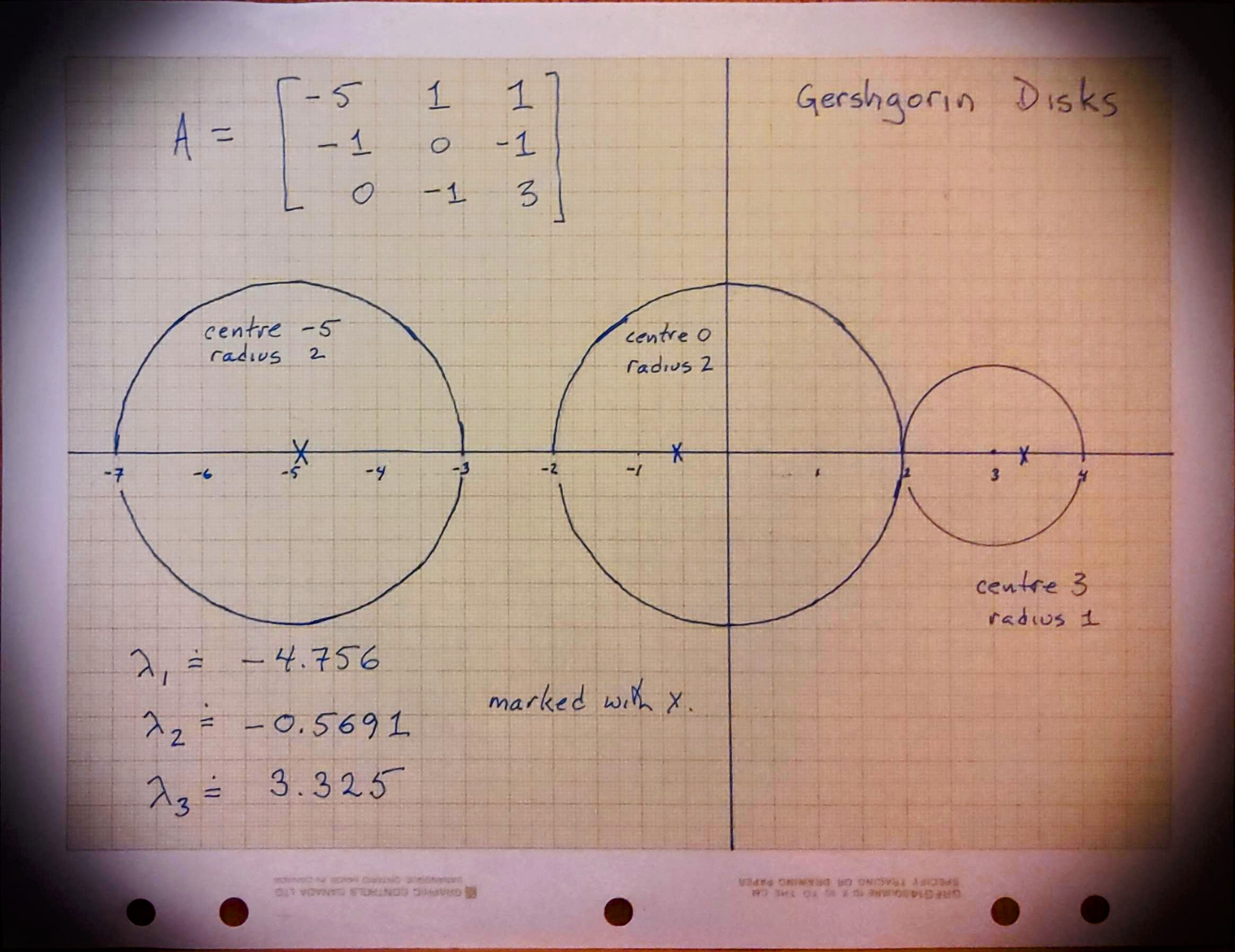
Fig. 14 A hand-drawn set of Gerschgorin disks#
Bohemian Activity 4#
Consider the matrix
Without computing the eigenvalues, can you decide if all of them are positive? Do you think it’s at least possible?
The matrix is symmetric so all its eigenvalues are real.
The Gerschgorin disks are all centred at \(2\). Two of them have radius \(1\), but both are inside the biggest one which has radius \(2\). This disk just touches \(0\) so it is at least in theory possible for an eigenvalue to be zero (and therefore not positive). We haven’t remarked on the fact that an eigenvalue equal to zero makes a matrix singular; the determinant is zero in that case. We can separately compute the determinant to show that it is not zero, and so all eigenvalues must be positive. But that’s somehow cheating, because we had to do a computation. Can we show that the matrix is nonsingular without computing a determinant? Another way to think about it (possible for people who have had linear algebra classes) is to try to write the middle column as a linear combination of the first and third (which are pretty clearly independent). This leads quickly to a contradiction, though: \(2\alpha = -1\), \(-2\alpha -2\beta = 2\), and \(2\beta = -1\) cannot all hold. Therefore the matrix is nonsingular because it has three independent columns.
Bohemian Activity 5#
Choose a matrix of your own (make it non-symmetric, with different radii from the theorem by rows than columns) and draw its Gershgorin circles and plot its eigenvalues.
We chose
We drew them out on graph paper that RMC has had for more than forty years and took pictures using Office Lens and added a “vintage” filter.
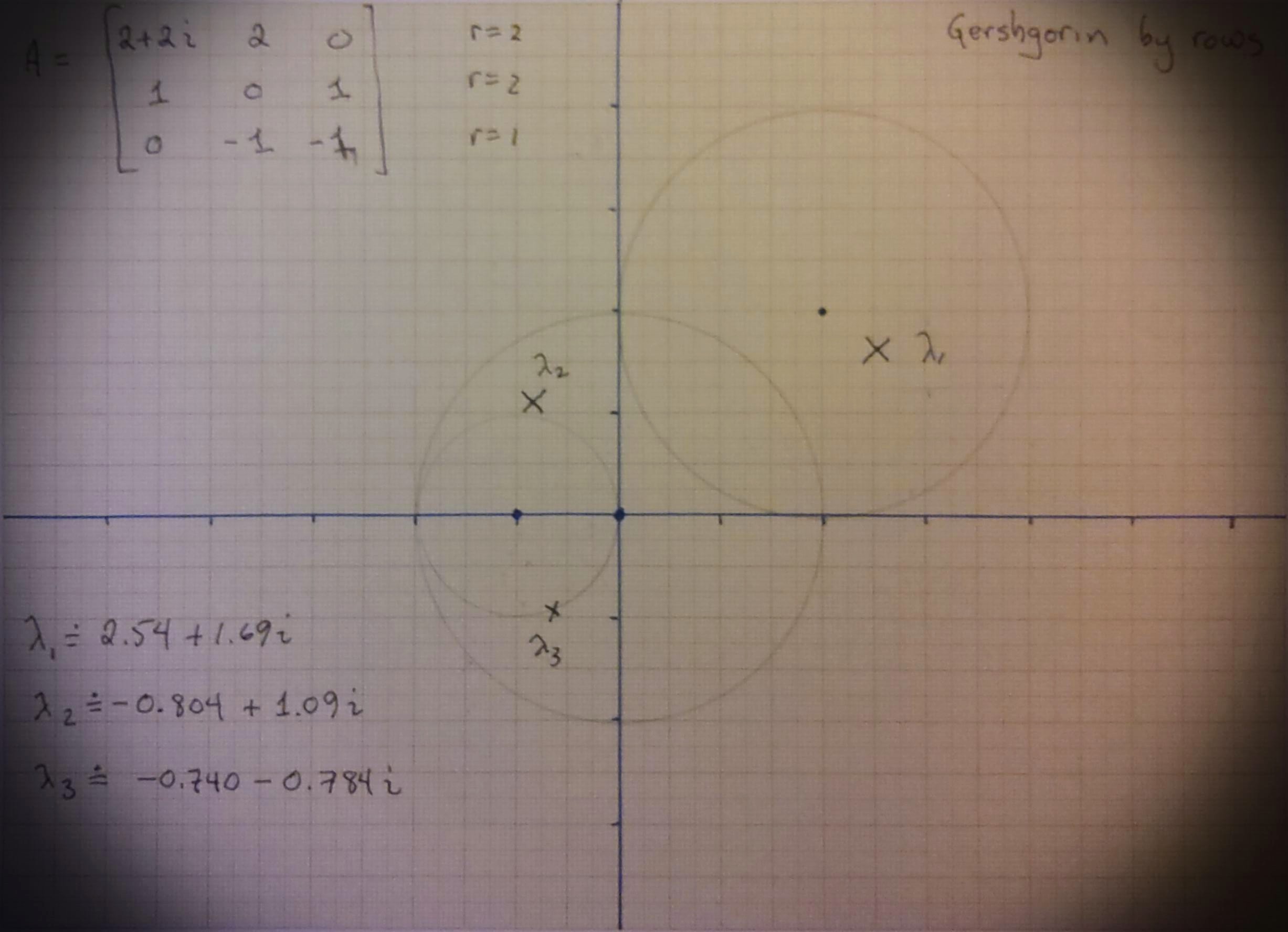
Fig. 15 A hand-drawn set of Gerschgorin disks, radii from the rows of the matrix#
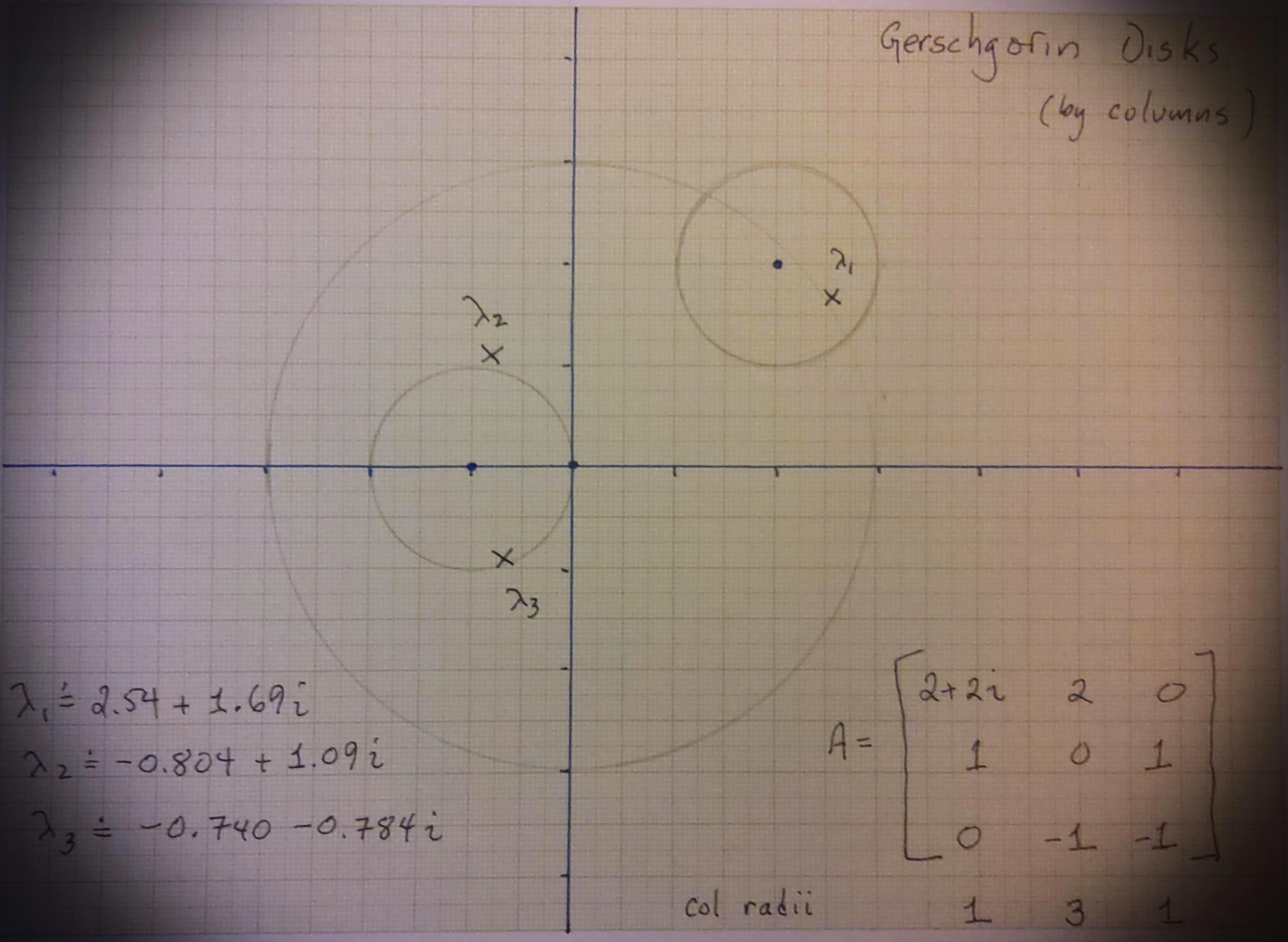
Fig. 16 A hand-drawn set of Gerschgorin disks, where the radii are from the columns. Here the union is not very different.#
Bohemian Activity 6#
“Can you see any other interesting features of this graph? What questions would you ask? Write some down. What other Bohemian questions can you think of?”
Maybe this is the most important one of these in this OER. Your questions are as likely as ours to be productive. But, here are some of ours. Most have no answers that we know of. In no particular order, here we go. For a given integer polynomial, which companion Bohemian matrix has minimal height? Which matrix in the family has the maximum determinant? Which matrix in the family has the maximum characteristic height? Minimum nonzero determinant? How many matrices are singular? How many are stable? How many have multiple eigenvalues? How many nilpotent matrices are there? How many non-normal matrices are there? How many commuting pairs are there? What is the distribution of eigenvalue condition numbers? How many different eigenvalues are there? How many matrices have a given characteristic polynomial? How many have nontrivial Jordan form? How many have nontrivial Smith form? How many are orthogonal? unimodular? How many matrices have inverses that are also Bohemian? With the same height? (In this case we say the matrix family has rhapsody). Given the eigenvalues, can we find a matrix in the family with those eigenvalues?
The colouring scheme we eventually settled on uses an approximate inversion of the cumulative density function and maps that onto a perceptually uniform sequential colour map like viridis or cividis. We have only just begun to explore more sophisticated schemes, but this one has the advantage that you can sort of “see” the probability density in the colours. Are there better methods? Can we do this usefully in \(3D\)? What about multi-dimensional problems? Tensors?
Bohemian Activity 7#
Change the population to various things in the list above and run that code yourself for various modest dimensions. Is the code correct? How could you tell? (If you do find a bug, please let us know!) Of the ones you tried, which population gives the fewest distinct characteristic polynomials? Which gives the most?
import itertools
import random
import numpy as np
from numpy.polynomial import Polynomial as Poly
import matplotlib as plt
import time
import csv
import math
from PIL import Image
import json
import ast
import sys
sys.path.insert(0,'../../code/Bohemian Matrices')
from bohemian import *
from densityPlot import *
populationlist = [complex(0,0),complex(1,0),complex(1, 1),complex(0, 1),complex(-1, 1),complex(-1,0),complex(-1, -1),complex(0, -1),complex(1, -1),
                               complex(2,0),complex(2, 1),complex(2, 2),complex(1, 2),complex(0, 2),complex(-1, 2),complex(-2, 2),complex(-2, 1),
                               complex(-2,0),complex(-2, -1),complex(-2, -2),complex(-1, -2),complex(0, -2),complex(1, -2),complex(2, -2),complex(2, -1)]
mdim = 2
A = Bohemian(mdim)
pcode = [10,15] # Code from the above figure: indexes into populationlist which was defined above.
population = [populationlist[p] for p in pcode]
print("The population is ", population)
sequencelength = A.getNumberOfMatrixEntries()
numberpossible = len(population)**sequencelength  # Each entry of the sequence is one of the population
# Generate (one at a time) all possible choices for
# vector elements: this is what itertools.product does for us.
possibilities = itertools.product(population, repeat=sequencelength)
possible = iter(possibilities)
# We will count the number of unique characteristic polynomials.
charpolys = {}
maxcount = 0
start = time.time()
for p in possibilities:
    A.makeMatrix(p)
    cp = tuple(A.characteristicPolynomial())
    if cp in charpolys.keys():
        charpolys[cp] += 1
        if charpolys[cp]>maxcount:
            maxcount = charpolys[cp]
            mostcommon = cp
            pattern = p
    else:
        charpolys[cp] = 1
finish = time.time()
print("Program took ", finish - start, " seconds \n")
print("There are ", len(charpolys), "distinct characteristic polynomials, vs ", len(population)**sequencelength, "matrices")
print("A most common characteristic polynomial was ", mostcommon, "which occurred ", maxcount, "times ")
A.makeMatrix(pattern)
print("One of its matrices was ",A.getMatrix())
The population is  [(2+1j), (-2+2j)]
Program took  0.0024292469024658203  seconds

There are  9 distinct characteristic polynomials, vs  16 matrices
A most common characteristic polynomial was  ((-0+0j), (-0-3j), (1+0j)) which occurred  4 times
One of its matrices was  [[-2.+2.j -2.+2.j]
 [ 2.+1.j  2.+1.j]]
With the population code [5,0] the population is \(\{-1,0\}\). This should give identical results to the population code [0,1] which should give the population \(\{0,1\}\), because we just multiplied all the matrices by \(-1\). The same with code [0,3] which multiplies by \(j\). When we ran the above code with those three populations, the number of distinct characteristic polynomials was the same each time, which increased our confidence. Also, the eigenvalues of the sample matrix returned (done separately from this notebook) were the same as the roots of the characteristic polynomial. Again this increased the confidence.
Giving it an unexpected population \(\{0,0\}\) made it count 16 different mdim=2 matrices (but really they were the same) though it correctly deduced there was only one characteristic polynomial. Is that a bug? We don’t think so. If the user calls the routine with unexpected input, getting weird output is the expected result!
Of the ones we tried here, the population \(2+j, -2+2j\) produced \(9\) distinct characteristic polynomials.
Some points for the Final Activities#
16. Looking back at the Fractals Unit, there seem to be clear connections with this unit. Discuss them.
Some of the Bohemian eigenvalue pictures are suggestive of fractals, especially the upper Hessenberg zero diagonal Toeplitz ones. In fact we have just managed to prove that Sierpinski-like triangles genuinely appear in some of these (when the population has three elements). In some other cases we think we have also managed to prove that in the limit as \(m\to\infty\) we get a genuine fractal. We can’t think of a way to connect the Julia set idea, though.
17. Looking back at the Rootfinding Unit, there seem to be clear connections with this unit. Discuss them.
Mostly the connection is practical: we want a good way to find all the roots of the characteristic polynomial (when we go that route, possibly because of the compression factor). Newton’s method can be used (sometimes!) to “polish” the roots to greater accuracy, for instance.
18. Looking back at the Continued Fractions Unit, it seems a stretch to connect them. Can you find a connection?
One connection: We thought of taking a general matrix and letting its entries be the partial quotients of the continued fraction of a number chosen “at random” in \([0,1)\). To make that “at random” have the right distribution turned out to be simple enough, because the distribution of partial quotients is known (called the Gauss-Kuzmin distribution) and its relation to the probability distribution of the iterates \(x_n\) of the Gauss map is also known (and called the “Gauss measure”). This is
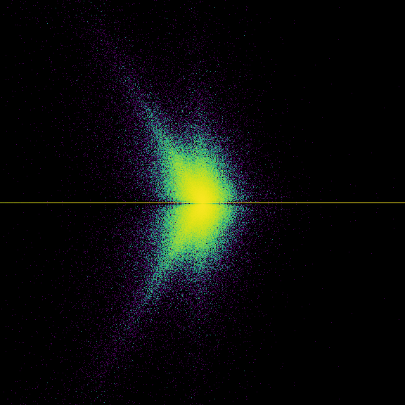
where the symbol lg means “log to base 2” and is frequently seen in computer science. We can invert this cumulative distribution by solving \(u=\mathrm{lg}(1+x)\) by raising both sides to the power \(2\), like so: \(2^u = 1+x\) so \(x=2^u-1\). Therefore, sampling \(u\) uniformly on \((0,1)\) will give \(x\) distributed on \((0,1)\) according to the Gauss measure; then taking the fractional part of \(1/x\) will give us the partial quotients with the correct distribution.
Doing this a large number of times and plotting the eigenvalue density we get a very interesting image; we’re still thinking about it. We were surprised that there was a pattern, and we don’t yet know how to explain it. This isn’t quite a Bohemian matrix problem, because the partial quotients of most numbers are unbounded. Still, very large entries are not likely, even though this is quite definitely what is known as a “heavy-tailed distribution” or “fat-tailed distribution”. The expected value of a partial quotient is infinity! The use of floating-point essentially bounds the largest entry in practice; we do not know what this does to the statistics.
Another way to connect continued fractions to Bohemian matrices might be to compute the continued fractions of the eigenvalues of one of our earlier computations, and see if there was any correlation with the “holes” (there might be—we have not tried this).
import itertools
import random
import numpy as np
from numpy.polynomial import Polynomial as Poly
import matplotlib as plt
import time
import csv
import math
from PIL import Image
import json
import ast
import sys
sys.path.insert(0,'../../code/Bohemian Matrices')
from bohemian import *
from densityPlot import *
rng = np.random.default_rng(2022)
# We will convert uniform floats u on (0,1) to
# floats that have the Gauss measure by x = 2^u - 1
# and this will get the right distribution of partial quotients

# This lambda function replaced by broadcast operations which are faster
# partial_quotient = lambda u: math.floor( 1/(2**u-1)) # u=0 is unlikely

# 5000 in 1.5 seconds, 50,000 in 12 seconds, 500,000 in 2 minutes, 1 million in 4 minutes
# six hours and 14 minutes for one hundred million matrices at mdim=13
Nsample = 1*10**5
mdim = 6
A = Bohemian(mdim)
sequencelength = A.getNumberOfMatrixEntries()
one = np.ones(sequencelength)
two = 2*one
start = time.time()
B =  0.6*mdim*(Nsample)**(0.25)
print( "Bounding box is width 2*{}".format(B))
bounds = [-B,B,-B,B] # Found by experiment; Depends on Nsample!
nrow = math.floor(9*B)  # These need to be adjusted depending on Nsample as well
ncol = math.floor(9*B)
image = DensityPlot(bounds, nrow, ncol)
for k in range(Nsample):
    u = rng.random(size=sequencelength)
    r = np.power(two,u)-one
    p = np.floor_divide(one,r)
    A.makeMatrix( p )
    image.addPoints(A.eig())

# We encode the population into a label which we will use for the filename.
poplabel = "ContinuedFraction"
cmap = 'viridis'
fname = '../Supplementary Material/Bohemian/dense/pop_{}_{}_{}N{}.png'.format(poplabel,cmap,mdim,Nsample)
image.makeDensityPlot(cmap, filename=fname, bgcolor=[0, 0, 0, 1], colorscale="cumulative")
finish = time.time()
print("Took {} seconds to compute and plot ".format(finish-start))
Bounding box is width 2*64.01805876140122
Took 14.295443773269653 seconds to compute and plot