Reports on Fibonacci Activities
Contents
Reports on Fibonacci Activities#
Fibonacci Activity 1#
The activity was to create the cells, input the numbers and the + sign into them, make sure it’s a “Code” cell, then hold down the CTRL (Command) key and hit ENTER to have the addition executed.
1
1
0+1
1
1+1
2
1+2
3
2+3
5
3+5
8
5+8
13
8+13
21
13+21 # One more than was asked for
34
One question we want to always ask about what a computer does, is “Are those results correct?” The answer here is yes, obviously, because we actually know these numbers from prior work and we can see that they are right. Of course we expect computers to get arithmetic right! But see the results in Activity 10. One good place to check sequence answers in general is at the Online Encyclopedia of Integer Sequences (OEIS), and of course the OEIS knows the Fibonacci numbers: sequence A000045. There are also good historical notes given there.
Fibonacci Activity 2#
Write a “for” loop in Python to compute the Lucas numbers up to \(L_{30}\). Compare your answers with the numbers given at the OEIS entry linked above (A000032).
Lucas_List = [2,1]
for i in range(2,31):
    nxt = Lucas_List[i-1]+Lucas_List[i-2]
    Lucas_List.append(nxt)
print(Lucas_List)
[2, 1, 3, 4, 7, 11, 18, 29, 47, 76, 123, 199, 322, 521, 843, 1364, 2207, 3571, 5778, 9349, 15127, 24476, 39603, 64079, 103682, 167761, 271443, 439204, 710647, 1149851, 1860498]
From the Online Encyclopedia of Integer Sequences, sequence A000032, we have that the Lucas sequence starts off with 2, 1, 3, 4, 7, 11, 18, 29, 47, 76, 123, 199, 322, 521, 843, 1364, 2207, 3571, 5778, 9349, 15127, 24476, 39603, 64079, 103682, 167761, 271443, 439204, 710647, 1149851, 1860498, 3010349, 4870847, 7881196, 12752043, 20633239, 33385282, 54018521, 87403803 . The output of the program above agrees, as far as it goes.
Fibonacci Activity 3#
Use a “while” loop to compute the Lucas numbers up to \(L_{30}\) using Python.
Lucas_List = [2,1]
i = 2
while i<31:
    nxt = Lucas_List[i-1]+Lucas_List[i-2]
    Lucas_List.append(nxt)
    i += 1
print(Lucas_List)
[2, 1, 3, 4, 7, 11, 18, 29, 47, 76, 123, 199, 322, 521, 843, 1364, 2207, 3571, 5778, 9349, 15127, 24476, 39603, 64079, 103682, 167761, 271443, 439204, 710647, 1149851, 1860498]
The output is exactly the same as before.
Fibonacci Activity 4#
The so-called Narayana cow’s sequence has the recurrence relation \(a_n = a_{n-1} + a_{n-3}\), with the initial conditions \(a_0 = a_1 = a_2 = 1\). Write a Python loop to compute up to \(a_{30}\). Compare your answers with the numbers given at the OEIS entry linked above (A000930).
Narayana_cows = [1,1,1]
for i in range(3,31):
    nxt = Narayana_cows[i-1] + Narayana_cows[i-3]
    Narayana_cows.append(nxt)
print(Narayana_cows)
[1, 1, 1, 2, 3, 4, 6, 9, 13, 19, 28, 41, 60, 88, 129, 189, 277, 406, 595, 872, 1278, 1873, 2745, 4023, 5896, 8641, 12664, 18560, 27201, 39865, 58425]
Comparing with the initial numbers at the OEIS entry for A000930, namely, 1, 1, 1, 2, 3, 4, 6, 9, 13, 19, 28, 41, 60, 88, 129, 189, 277, 406, 595, 872, 1278, 1873, 2745, 4023, 5896, 8641, 12664, 18560, 27201, 39865, 58425, 85626, 125491, 183916, 269542, 395033, 578949, 848491, 1243524, 1822473, 2670964, 3914488, 5736961, 8407925, we see that the numbers are the same, as far as they go.
Fibonacci Activity 5#
Write Python code to draw the traditional Fibonacci Spiral.
A google search turns up the following Turtle Geometry in Python Fibonacci Spiral by DavisMT, which is a bit more advanced than we had in mind; but it suffices. There are lots of others to choose from. Discussion of which is best could be a nice classroom activity.
Fibonacci Activities 6 and 7#
We invented something that we think is new! The activity for you was, Write a Python program to draw these triangles and draw a spiral line through the resulting Fibonacci numbers (starting at 2).
For the new spiral, we need a bit of pen-and-paper work first to work out the angles, and a consistent numbering scheme. If we make one vertex of each triangle be the origin, it makes a nice picture with the triangles successively touching each other. In this case it will work out better if we draw the picture first, then explain the code that drew the picture.
# Isosceles Fibonacci Triangle Spiral
Final_Triangle = 7  # We will draw triangles from the flat one on, and stop at a "Final Triangle"
# We will need one more Fibonacci number than triangles (because we throw the first one away )
Fibonacci = [0,1]
for i in range(2,Final_Triangle+2):
    nxt = Fibonacci[i-1]+Fibonacci[i-2]
    Fibonacci.append(nxt)
angle_cosines = [Fibonacci[i]/(2*Fibonacci[i-1]) for i in range(3,Final_Triangle+2)]

# When writing this code, print statements like the following
# were very useful for debugging.  We have left them in, but commented them out
# so Python does not execute them (but you can see them)
# print( angle_cosines )

import numpy as np

# These are the small angles in the isosceles triangles
angles = [np.arccos(t) for t in angle_cosines ]

print(angles)  # Actually there is something interesting about these angles
print(np.pi/5)

# We need the cumulative sums of those angles for our spiral
theta = np.cumsum(angles)

#print(theta)
r = [Fibonacci[i] for i in range(3,Final_Triangle+2)]
#print(r, r[-1])

import matplotlib.pyplot as plt

fig, ax = plt.subplots(subplot_kw={'projection': 'polar'}) # same as before
# Plot the spiral (ie the outermost points of each triangle)
ax.plot(theta, r) # same as before

# Now plot the long sides of each triangle
for i in range(len(r)):
    ax.plot([0,theta[i]], [0, r[i]])

ax.set_rmax(r[-1]) #
ax.set_rticks(r)  # Show Fibonacci radii for our plot
#ax.set_rlabel_position(-22.5)  # don't need this command
ax.grid(True) # same as before

ax.set_title("New Fibonacci Spiral", va='bottom') # change the title
plt.show()
[0.0, 0.7227342478134157, 0.5856855434571508, 0.6435011087932843, 0.6223684885550206, 0.630568739599553]
0.6283185307179586
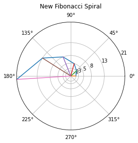
There’s lots to talk about in that code. The “cumsum” function has an odd name (the same name as the corresponding function in Matlab) but it just replaces a list [x, y, z, w] with another list [x, x+y, x+y+z, x+y+z+w]. So, simple but useful. We needed it because the direction the final triangle is pointing has as its angle the sum of its internal angle plus all the angles of the previous triangles: the cumulative sum, in other words. The final entry in a list can be referred to by asking for the “-1” entry, viz: r[-1] gives us the largest radius. The counting was hard, because there is no (0,0,1) triangle, and the (1,1,2) triangle is flat and has internal angles 0 or 180 degrees (0 or \(\pi\) radians, and of course the trig functions in Python use radians). Python chose the colours of the lines, because we didn’t specify them; the labels are a bit squashed up because we didn’t try very hard to make this spiral pretty. We expect that you can already do better than this program.
We did not try to draw a smooth curve through the points, but a polar curve with radius \(\phi^t/\sqrt{5}\) and angle linear in \(t\) can be made to match these points pretty closely. That’s also not a bad activity.
The interesting fact alluded to above, when we printed the angles, was that they very quickly settle down to \(\pi/5\). This is because \(F_n/(2F_{n-1})\) very quickly settles down to \(\phi/2\), and, which is a surprising fact, the angle whose cosine is \(\phi/2\) is \(\pi/5\). There is a square root of 5 in \(\phi\), and a \(5\) in the radian measure of its arccosine; is this a coincidence? You might want to try to prove to yourself that these facts are true; if you manage it, you might simultaneously find a reason (or alternatively decide that it is, in fact, just a coincidence). But that sort of thing is much more like traditional math, and so we reluctantly do not pursue it here.
Fibonacci Activities 8 and 9#
Now we look at the activities with the length (in bits) of Fibonacci numbers. The first question is “Compute the \(n\)th Fibonacci number for \(n=100\), \(1000\), and \(10000\). How many digits does each have? Can you predict the number of digits in \(F_n\) as a function of \(n\)? How many bits in the binary expansions? “
First we check that Binet’s formula does a reasonable job:
phi = (1+np.sqrt(5))/2
def Binet(n):
    return(np.round( phi**n / np.sqrt(5)))

print(Binet(1), Binet(2), Binet(3), Binet(4), Binet(5), Binet(6), Binet(7))
print(Binet(10), Binet(100), Binet(1000))
1.0 1.0 2.0 3.0 5.0 8.0 13.0
55.0 3.542248481792631e+20 4.3466557686938915e+208
def fibo(n):
    prev = 0
    curr = 1
    for i in range(2,n+1):
        fib = curr + prev
        prev = curr
        curr = fib
    return(fib)

print(fibo(10), fibo(100), fibo(1000), fibo(1000))
55 354224848179261915075 43466557686937456435688527675040625802564660517371780402481729089536555417949051890403879840079255169295922593080322634775209689623239873322471161642996440906533187938298969649928516003704476137795166849228875 43466557686937456435688527675040625802564660517371780402481729089536555417949051890403879840079255169295922593080322634775209689623239873322471161642996440906533187938298969649928516003704476137795166849228875
Those numbers agree (up to floating-point error) and so we accept the formula \(F_n \approx \phi^n/\sqrt{5}\). Since we are told that the length (in bits) of \(F_n\) has something to do with \(\log_2 F_n\), we think for a moment and realize that it actually takes \(\lceil \log_2 F_n \rceil\) bits, where the ceiling of a real number \(x\), namely \(\lceil x \rceil\), is defined as the integer you get when you round up (alternatively, it is the smallest integer greater than or equal to \(x\)). Now we try to simplify
(We ignored the \(-\log_2\sqrt{5}\) in that last line because that is only about 1 bit, and if \(n\) is at all large, that \(1\) won’t matter.) By simple computation, we have \(\ln \phi/\ln 2 \approx 0.4812/0.6931 \approx 0.6942 \). This predicts that the number of bits needed to represent \(F_n\) should be linearly related to \(n\), at least approximately. Let’s try first for \(F_{10} = 55\). In binary, this is \(110111\), which needs six bits. The prediction, on the other hand, is \(0.6942\cdot 10 = 6.942\), either \(6\) or \(7\) bits. This is adequate agreement, but not convincing. Now let’s try \(F_{100} = 354224848179261915075\) which took 69 bits; the prediction is \(69.42\) bits, which is better agreement. Converting \(F_{1000}\) to binary gives \(1000011101100011001011000001111011010101110010110000100101011100110010101110110001000101101111001011000011001110111010101100001110100000111101000011000110100110011011101011010001101001110010011110100111001101101010011111100100001011001010100100111011011010010111101011010010001001001101010101010011100110000011011100110000011000101111000110001111111101100010101110011001110000101000000001101000000100110001101000111111101010110000110000010010111000110101000100000010100000111100000111010110000010110000000010010011000010110111111010001000000000111100001100010010101101001100100011100110110101010010100001101000000001011111110001110000101101011001010011011100011101011100110000000110000001001011\) which has \(694\) bits. We hope that this is convincing, now.
print(np.log(5)/(2*np.log(2))) # log base 2 of the square root of 5
1.160964047443681
bin(fibo(1000))
'0b1000011101100011001011000001111011010101110010110000100101011100110010101110110001000101101111001011000011001110111010101100001110100000111101000011000110100110011011101011010001101001110010011110100111001101101010011111100100001011001010100100111011011010010111101011010010001001001101010101010011100110000011011100110000011000101111000110001111111101100010101110011001110000101000000001101000000100110001101000111111101010110000110000010010111000110101000100000010100000111100000111010110000010110000000010010011000010110111111010001000000000111100001100010010101101001100100011100110110101010010100001101000000001011111110001110000101101011001010011011100011101011100110000000110000001001011'
len(bin(fibo(1000)))
696
That length is 696 and not 694 because of the extra two characters ‘0b’ at the start.
a = bin(0)
print(a[0],a[1], a[2], a,
      a[-1])
0 b 0 0b0 0
Fibonacci Activity 10#
Figure out how to implement iterated squaring to compute \(A^{51}\) by a sequence of Python statements. Then code a function which will take \(n\) and \(A\) as inputs, compute \(A^n\) by iterated squaring (also called binary powering and the general strategy is sometimes called “divide and conquer”) and return it.
You should only need to use two matrices for storage if you are careful. There are several ways to do this. For one method, a hint is to find the low order bits of \(n\) first.
def bipow(A, n):
    ndim = A.shape[0]
    ni = n
    answer = np.identity(ndim, dtype=int)
    multiplier = A
    # At this point, with ni = n, we have A**n = answer*multiplier**ni
    while ni > 0:
        # print(binaryn[-i])
        if ni % 2 == 0:
            # Even bit, so ni <- ni/2
            ni = ni/2 # Integer division
            multiplier = np.matmul(multiplier,multiplier)
            # Still true that answer*multiplier**ni = A**n
        else:
            # Odd bit, so ni <- ni - 1
            ni = ni - 1
            answer = np.matmul(answer,multiplier)
            # Still true that answer*multiplier**ni = A**n
    return(answer) # At this point, ni=0 so answer = A**n
Let us prove, by induction on \(n\), that the code above is correct, on the assumption that the inputs are a matrix A and a nonnegative integer \(n\).
At the first marked point, the variables “answer” and “multiplier” and “ni” are such that
A**n = answer*multiplier**ni.The while loop terminates with ni=0. To prove this, note that every time through the loop ni is replaced by a smaller integer, either ni/2 or ni-1. Therefore the loop executes a finite number of times. It only terminates if ni=0.
After each branch of the if statement, it remains true that
A**n = answer*multiplier**ni. This is a “loop invariant”. This is because in the “even” branch, the multiplier is squared soA**n = answer*(multiplier**2)**(ni/2), and in the “odd” branch the answer variable is altered soA**n = (answer*multiplier)*(multiplier**(ni-1)).When the loop ends, ni=0, so “answer” contains
A**n.
A = np.array([[1,1],[-1,1]])
B = np.matmul(np.matmul(A,A), A)
print(A, B, bipow(A,3))
[[ 1  1]
 [-1  1]] [[-2  2]
 [-2 -2]] [[-2  2]
 [-2 -2]]
The statements below are a kind of “minimal test” of the code above. The difference between \(A^n\) computed by one method versus bipow(A,n) should be zero, and for our examples, it is. Even though the code contains a proof of correctness using “loop invariants” and induction, one wants to test the code. By using a random matrix and a bunch of powers, both odd and even, one gains some confidence.
That code did not run correctly the first time, either! Even though RMC has been programming for decades, and has written this particular program before in other languages, there were glitches, now fixed. To find and fix the glitches, he inserted various print statements to look at intermediate results. Eventually he gave up on using the binary expansion of n to decide whether to square or to multiply because it was too “fiddly” and changed to the more straightforward method above. This code is easier to read, if marginally less efficient. We tell you this just to let you know that writing code involves dealing with bugs, and that this is always an issue.
A = np.random.randint(-99,99,(10,10))
A2 = np.matmul(A,A)
A4 = np.matmul(A2,A2)
A3 = np.matmul(A2,A)
A7 = np.matmul(A4,A3)
print(bipow(A,2)-A2, bipow(A,3)- A3, bipow(A,4)- A4, bipow(A,7)- A7)
[[0 0 0 0 0 0 0 0 0 0]
 [0 0 0 0 0 0 0 0 0 0]
 [0 0 0 0 0 0 0 0 0 0]
 [0 0 0 0 0 0 0 0 0 0]
 [0 0 0 0 0 0 0 0 0 0]
 [0 0 0 0 0 0 0 0 0 0]
 [0 0 0 0 0 0 0 0 0 0]
 [0 0 0 0 0 0 0 0 0 0]
 [0 0 0 0 0 0 0 0 0 0]
 [0 0 0 0 0 0 0 0 0 0]] [[0 0 0 0 0 0 0 0 0 0]
 [0 0 0 0 0 0 0 0 0 0]
 [0 0 0 0 0 0 0 0 0 0]
 [0 0 0 0 0 0 0 0 0 0]
 [0 0 0 0 0 0 0 0 0 0]
 [0 0 0 0 0 0 0 0 0 0]
 [0 0 0 0 0 0 0 0 0 0]
 [0 0 0 0 0 0 0 0 0 0]
 [0 0 0 0 0 0 0 0 0 0]
 [0 0 0 0 0 0 0 0 0 0]] [[0 0 0 0 0 0 0 0 0 0]
 [0 0 0 0 0 0 0 0 0 0]
 [0 0 0 0 0 0 0 0 0 0]
 [0 0 0 0 0 0 0 0 0 0]
 [0 0 0 0 0 0 0 0 0 0]
 [0 0 0 0 0 0 0 0 0 0]
 [0 0 0 0 0 0 0 0 0 0]
 [0 0 0 0 0 0 0 0 0 0]
 [0 0 0 0 0 0 0 0 0 0]
 [0 0 0 0 0 0 0 0 0 0]] [[0 0 0 0 0 0 0 0 0 0]
 [0 0 0 0 0 0 0 0 0 0]
 [0 0 0 0 0 0 0 0 0 0]
 [0 0 0 0 0 0 0 0 0 0]
 [0 0 0 0 0 0 0 0 0 0]
 [0 0 0 0 0 0 0 0 0 0]
 [0 0 0 0 0 0 0 0 0 0]
 [0 0 0 0 0 0 0 0 0 0]
 [0 0 0 0 0 0 0 0 0 0]
 [0 0 0 0 0 0 0 0 0 0]]
Now let’s use this to generate Fibonacci numbers. At first, all goes well, but when we tried to find \(F_{51}\) by this method, we got a shock. On one of our systems, the following code produced the output quoted below the cell below:
A = np.array([[1,1],[1,0]])
print(bipow(A,4))
print(bipow(A,5))
print(bipow(A,30))
print(bipow(A, 51))
[[5 3]
 [3 2]]
[[8 5]
 [5 3]]
[[1346269  832040]
 [ 832040  514229]]
[[32951280099 20365011074]
 [20365011074 12586269025]]
Quoting that answer for posterity (copied-and-pasted into a Markdown version, showing what happened when this code was run on RMC’s machine):
[[5 3]
 [3 2]]
[[8 5]
 [5 3]]
[[1346269  832040]
 [ 832040  514229]]
[[-1408458269 -1109825406]
 [-1109825406  -298632863]]
Now we see a truly staggering thing about computers and programs. We proved our program was correct. We tested our program. And now we see that it can give wrong results! There is no way that raising the Fibonacci matrix to a positive power can produce a matrix with negative entries.
Maybe even worse, your system may not have given the same answer. Maybe the answer on your system was correct!
What on earth happened here? The answer is in the internal data structure. Let us look for the first time this happens.
print(bipow(A,40))
[[165580141 102334155]
 [102334155  63245986]]
print(bipow(A,45))
[[1836311903 1134903170]
 [1134903170  701408733]]
print(bipow(A,47))
[[4807526976 2971215073]
 [2971215073 1836311903]]
quoting that for posterity, because the output on your system may be different:
[[  512559680 -1323752223]
 [-1323752223  1836311903]]
print(bipow(A,46))
[[2971215073 1836311903]
 [1836311903 1134903170]]
again quoting that for posterity, because the output on your system may be different:
[[-1323752223  1836311903]
 [ 1836311903  1134903170]]
1836311903+1134903170
2971215073
That’s what that entry in the matrix should have been, not -1323752223. How could this happen?
len(bin(2971215073))
34
len(bin(1836311903))
33
For Linux/Unix systems, our program fails at \(n=92\).
print(bipow(A,92))
[[-6246583658587674878  7540113804746346429]
 [ 7540113804746346429  4660046610375530309]]
It turns out that there is such a thing as a thirty-two bit signed integer. The leading bit of that kind of integer is 0 if the number is positive, but if the leading bit is 1 then the number is taken to be negative. Thus, on a computer, if the wrong datatype is used, it is possible to add two positive integers and have the result be interpreted as being negative.
And there is the problem. Remember that the length of a binary number includes the “0b” at the beginning, so the number that wound up being negative was 32 bits long; whereas the last Fibonacci number that was ok was 31 bits long. Somehow the code decided that it was using “32 bit integers” instead of the normal Python arbitrary-length integers. Our “proof” assumed the normal properties of integers—which are needed for the matrix multiplication to be correct—and this kind of assumption is so natural to us we didn’t even notice we used it.
Welcome to the world of computer programming. Yes, we have to know about data types.
In this particular case, it is even more problematic that the issue appears only on some machines (on Windows but not on Linux, for instance). Welcome to the world of computing on shifting sand, where versions matter, where the particular computer matters, and complexity is an ever-growing issue.
Here is a discussion of the issue
Moreover, it is possible that this behaviour could change in future. Nonetheless, that this artifact existed at one time may give you pause in believing the output of computer systems uncritically.
We could fix this by writing our own matrix multiply that uses Python long integers (its default) instead of NumPy’s 32 bit integers, and perhaps that’s a useful activity. We will leave that to linear algebra class though. Instead we will look a bit more carefully at just what we need here; and we will do so in the main text, not here in the “Report” section. Instead we just provide (with very little comment) a report for the “divide and conquer” suggested advanced activity. This code is recursive (but not exponentially expensive), uses “tuples” (the pairs of numbers (\(F_{n-1},F_n\)) ) and recurrence relations derived from the matrix multiplication described in the main text. It also does not use NumPy and therefore winds up using the default Python long integers, so we get correct answers (provided we don’t call it with zero, or negative integers, or nonsense).
def FibonacciByHalving(n):
    if n ==1 :
        return((0,1))
    else:
        m, r = divmod(n, 2)  # The quotient + remainder (either 0 or 1)
        fm1, fm = FibonacciByHalving( m ) # A problem of half the size
        if r==0:
            fn  = fm*(fm + 2*fm1)
            fn1 = fm*fm + fm1*fm1
        else:
            fn  = (fm+fm1)**2 + fm**2
            fn1 = fm*(fm + 2*fm1)
        return((fn1,fn))
FibonacciByHalving(47)
(1836311903, 2971215073)
import time
st = time.time()
FibonacciByHalving(1000000) # Took 10 seconds on this machine when using "fibo"
time_taken = time.time() - st
print(time_taken)
0.08402514457702637
So that code was more than a hundred times faster than the original “fibo” code. Not bad. What about for ten million? Twenty million? Remember, \(F_n\) has about 0.694n bits in it—so \(F_{10^7}\) will have more than six million bits; the answer is so large that dealing with it must take time.
st = time.time()
FibonacciByHalving(10**7) #
time_taken = time.time() - st
print(time_taken)
3.323323965072632
st = time.time()
FibonacciByHalving(2*10**7)
time_taken = time.time() - st
print(time_taken)
11.64668321609497
It looks like doubling the size of the input led to the computation taking roughly four times the time. (Somewhat annoyingly, the times reported are quite variable: on this run it was 3 seconds vs 13 seconds, but sometimes it’s 3 seconds vs 8 seconds, which looks better; to get accurate timings, one has to do many runs. We don’t do this here, because this is only rough work.) The factor of 4 (when we see it) seems like quadratic growth, which we were hoping to avoid: the cost seems proportional to \(n^2\). But this happens because multiplication is more expensive than addition; even though we are doing fewer operations, we are doing more expensive multiplication; and we have to multiply six million bit integers together, and that takes time.
We can fix this by using faster methods to multiply integers but that’s Python’s problem. They should implement the fast multiplication methods. That’s not our job.
Fibonacci Activity 11#
Which is a better method, using matrices or using Binet’s formula, to compute Fibonacci numbers up to (say) \(F_{200}\)? Does using the iterated squaring help with Binet’s formula as well? How many decimal digits do you have to compute \(\phi\) to in order to ensure that \(F_n\) is accurate? You don’t have to prove your formula for number of decimal digits, by the way; experiments are enough for this question. You will have to figure out how to do variable precision arithmetic in some way (perhaps by searching out a Python package to do it).
We have demonstrated that FibonacciByHalving, which is related to the matrix method, is better than either (it doesn’t waste space, for instance). While Binet’s formula is useful for a lot of things, the variable precision needed for large \(n\) (if one wants the exact answer) mean that it’s usually simpler to compute with (long) integers.
As for the precision question, in this case you get out what you put in. The length of the Fibonacci number that you get out has so many bits of precision, and you can’t get that from an inaccurate value of \(\phi\). The question of how much precision do you need is a bit tricky, though. By theoretical means (see the “Best Approximation” section at the end of the unit) we can deduce that \(F_{n+1}/F_n - \phi\) is about the same size as \(1/F_n^2\). This turns the problem on its head: if we could use low-accuracy versions of \(\phi\) to get a good \(F_n\), then we could turn around and improve the accuracy of \(\phi\). This seems like “something for nothing”. More prosaically, using 5 digits of \(\phi\) gets you the first five or so digits of \(F_n\), no more; this means that it’s good up to about \(n = 16\). When \(n=17\), \(F_n = 1597\) and \(F_n^2\) is bigger than a million, so \(1/F_n^2\) is smaller than \(10^{-6}\) and so computing an approximation to \(F_{17}\) from the five-digit \(\phi\) doesn’t work.
Fibonacci Activity 12#
Compute the last twenty digits of \(F_n\) where \(n = 7^{k}\) for \(k=1\), \(k=12\), \(k=123\), \(k=1234\), and so on, all the way up to \(k=123456789\), or as far as you can go in this progression using “reasonable computer time”. Record the computing times. At Clemson the student numbers are eight digits long, and these can be used in place of \(123456789\) in the progression above, for variety.
def FibonacciByHalvingModM(n,M):
    if n ==1 :
        return((0,1))
    else:
        m, r = divmod(n, 2)  # The quotient + remainder (either 0 or 1)
        fm1, fm = FibonacciByHalvingModM( m, M ) # A problem of half the size
        if r==0:
            fn  = (fm*(fm + 2*fm1)) % M  # Extra parens seem to be necessary
            fn1 = (fm*fm + fm1*fm1) % M
        else:
            fn  = ((fm+fm1)**2 + fm**2) % M
            fn1 = (fm*(fm + 2*fm1)    ) % M
        return((fn1,fn))
FibonacciByHalvingModM(10**6, 100)
(26, 75)
st = time.time()
FibonacciByHalvingModM(7**123,10**100)
time_taken = time.time() - st
print(time_taken)
0.0014760494232177734
#st = time.time()
#FibonacciByHalvingModM(7**1234,10**100)
#time_taken = time.time() - st
#print(time_taken)
Here’s the error message that occurs when that last cell is uncommented (remove the # from the start of each line)
RecursionError                            Traceback (most recent call last)
Input In [38], in <module>
      1 st = time.time()
----> 2 FibonacciByHalvingModM(7**1234,10**100)
      3 time_taken = time.time() - st
      4 print( time_taken )

Input In [35], in FibonacciByHalvingModM(n, M)
      4 else:
      5     m, r = divmod( n, 2 )  # The quotient + remainder (either 0 or 1)
----> 6     fm1, fm = FibonacciByHalvingModM( m, M ) # A problem of half the size
      7     if r==0:
      8         fn  = (fm*(fm + 2*fm1)) % M  # Extra parens seem to be necessary

    [... skipping similar frames: FibonacciByHalvingModM at line 6 (2969 times)]

Input In [35], in FibonacciByHalvingModM(n, M)
      4 else:
      5     m, r = divmod( n, 2 )  # The quotient + remainder (either 0 or 1)
----> 6     fm1, fm = FibonacciByHalvingModM( m, M ) # A problem of half the size
      7     if r==0:
      8         fn  = (fm*(fm + 2*fm1)) % M  # Extra parens seem to be necessary

Input In [35], in FibonacciByHalvingModM(n, M)
      1 def FibonacciByHalvingModM(n,M):
----> 2     if n ==1 :
      3         return( (0,1) )
      4     else:

RecursionError: maximum recursion depth exceeded in comparison
So, that recursive code cannot do the \(7^{12345678}\) version, or even \(7^{1234}\), because recursions are only allowed to nest so deep: the “stack” overflows. It’s not clear Python could even handle such a big input anyway, without testing. (But, it seems to work, as seen below). But to find the final 100 digits of the Fibonacci number for this \(n\), we’re going to have to work a bit harder to make it possible for the computer to get it.
st = time.time()
big = 7**12345678; # Has about 10 million digits when expanded.  Not sure Python gets it right.
time_taken = time.time() - st
print(time_taken)
13.795675992965698
# Manually translated from the Maple routine combinat[fibonacci]
def FibonacciByDoubling(n):
    if n==0:
        return(0)
    elif n<0:
        return( (-1)**(1-n)*FibonacciByDoubling(-n) )
    else:
        p = n
        b = []
        while p != 0:
            m, r = divmod( p, 2 )
            p    = m
            b.append(r)
        f0 = 0
        f1 = 1
        for i in range(len(b)-2,-1,-1):
            if b[i]==0:
                s = f0
                if i>0:
                    f0 = f1**2 + f0**2
                f1 = f1*(f1+2*s)
            else:
                s = f1
                f1 = f1**2 + (f0+f1)**2
                if i>0:
                    f0 = s*(s+2*f0)
        return(f1)
FibonacciByDoubling(20), FibonacciByHalving(20) # The answer should be the same, both ways, and it is.
(6765, (4181, 6765))
# Modular arithmetic folded in
def FibonacciByDoublingModM(n, M):
    if n==0:
        return(0)
    elif n<0:
        return( (-1)**(1-n)*FibonacciByDoublingModM(-n,M) )
    else:
        p = n
        b = []
        while p != 0:
            m, r = divmod( p, 2 )
            p    = m
            b.append(r)
        f0 = 0
        f1 = 1
        for i in range(len(b)-2,-1,-1):
            if b[i]==0:
                s = f0
                if i>0:
                    f0 = (f1**2 + f0**2) % M
                f1 = (f1*(f1+2*s)) % M
            else:
                s = f1
                f1 = (f1**2 + (f0+f1)**2) % M
                if i>0:
                    f0 = (s*(s+2*f0)) % M
        return(f1)
st = time.time()
Final100 = FibonacciByDoublingModM(7**123456,10**100)
time_taken = time.time() - st
print(time_taken, Final100)
25.377628803253174 3303961837047442579487010911533190161514152117063487274236115429253289173645117777960901109522457601
Now we seem to be “cooking with gas”! But the exponent we want is a hundred times larger, so we would have to do (it seems) vastly more work, impractically so. So, again, we need a better method, not just better programming skills.
Fibonacci Activity 13#
Compute the last hundred digits of \(F_n\) where \(n = 7^{12345678}\) for yourself, and confirm our answer (or prove us wrong).
We will need modular arithmetic for very high powers, and it looks like Python’s built-in code has some limitations. The following answer is, apparently, wrong. It is certainly not what we expected! Raising seven to a power gets an odd number, surely! In response, we wrote our own code. (But it turns out Python is “right”, it’s just doing something we didn’t expect—more after our own code).
PythonFailure = 7**12345678 % 15*10**99
print(PythonFailure)
4000000000000000000000000000000000000000000000000000000000000000000000000000000000000000000000000000
That can’t be right. It’s certainly not the answer Maple gets. Well, let’s write our own modular powering, using the same trick as is used in bipow above.
def BinaryIntegerPowerModM( a, b, M):
    n = b
    answer = 1
    multiplier = a % M
    while n > 0:
        if n % 2 == 0:
            n = n/2
            multiplier = multiplier * multiplier % M
        else:
            n = n - 1
            answer = answer * multiplier % M
    return(answer)
st = time.time()
good = BinaryIntegerPowerModM(7, 12345678, 15*10**99)
time_taken = time.time() - st
print(good, time_taken)
10074958745783517956561868690867278026860583978054601497639995184130970247153466763696198800985914449 0.0001227855682373047
That’s the same answer Maple got. It took us a while to understand Python’s different answer with direct use of %. We thought at first, possibly some kind of overflow of the long integer? It seemed that it computed the large number first and only then tried to do the modular computation. But, no. The problem was we need brackets. But, we learned (by checking the time taken) that Python indeed builds that ten-million-digit number first, and then uses modular arithmetic. Our code was quite a bit faster. (A factor of 1700 faster on one run, which makes us happy; the timings in this run may differ).
Now try nine digits.
st = time.time()
good = BinaryIntegerPowerModM( 7, 123456789, 15*10**99 )
time_taken = time.time() - st
print(good, time_taken)
9970146625619845782834561006870277384130667336988626592393064577383315981126385562996947892776429607 0.00013589859008789062
st = time.time()
PythonSucceeds = 7**12345678 % (15*10**99)
time_taken = time.time() - st
print(PythonSucceeds, time_taken)
10074958745783517956561868690867278026860583978054601497639995184130970247153466763696198800985914449 13.93323302268982
st = time.time()
ans = FibonacciByDoublingModM(10074958745783517956561868690867278026860583978054601497639995184130970247153466763696198800985914449,10**100)
time_taken = time.time() - st
print(ans, time_taken)
307317414528301264423288910092883733560870958520339896436368099936463847448493468403352592709652449 0.002080202102661133
st = time.time()
ans = FibonacciByDoublingModM(10074958745783517956561868690867278026860583978054601497639995184130970247153466763696198800985914449,10**10)
time_taken = time.time() - st
print(ans, time_taken)
2709652449 0.0006058216094970703
Fibonacci Activity 14#
Write down some questions (don’t worry about answers) about Fibonacci numbers or the Binet formula.
We really do want you to write your own questions. It’s likely that some of the questions you ask will not be productive (that’s true of the questions we write down, that’s how we know) but because you think about these things differently than we do your chance of coming up with a productive new question is not at all bad.
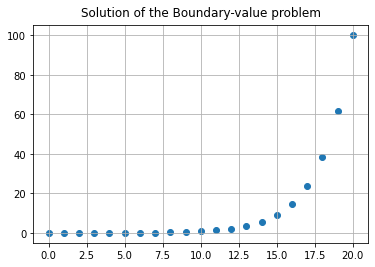
Here’s our free-association try at answering this. What happens if we replace the two initial conditions \(F_0 = 0\) and \(F_1=1\) with boundary conditions, say \(F_0=0\) and \(F_{20} = 100\)? What happens if you reverse the digits of the Fibonacci numbers? (0, 1, 1, 2, 3, 5, 8, 31, 12, 55, 98, \(\ldots\)). (We have no idea if that’s productive or not, but we bet “not”). What happens if you reverse the bits in the binary expansion? Is there any linear relation among the results? (Ok maybe it’s interesting). What happens if instead of always adding \(F_{n} + F_{n-1}\) one randomly chose between adding and subtracting? (This is quite likely a very interesting question). Is there a second order difference equation whose solutions grow more slowly than the Fibonacci numbers? How many papers have been written about Fibonacci numbers? How many books? Is there someone in the world who might be considered “the world’s greatest Fibonacci expert?” (Ok, now we’re getting silly.) What is the “most beautiful” Fibonacci image or sculpture? Is there Fibonacci-based music? (Apparently there is Sanskrit poetry that is related, so why not music?) What is the most practical use of the Fibonacci numbers? (Yes, there are some.) There are apparently some financial “uses” of Fibonacci numbers in trading: are those just another scam? Remember, caveat emptor.
Afterwards, choose out one of your questions and (if you want) answer it
We’ll take the “boundary value” question, because it’s connected with a number of other mathematical subjects. We could set this up as a linear system of equations, write down the matrix, and solve it that way. This connects the problem with linear algebra. But let’s take a step back, and use a (significantly!) older method, known as Ahmes’ method which we know from the Rhind papyrus. This also, in this context, connects with one method for solving boundary value problems for ordinary differential equations that you might meet in a later numerical methods class, but that’s just a bonus. Ahmes method is to guess what one unknown is, then solve the problem that way, then linearly adjust the guess so that your answer works out correctly. We will use it in a slightly more systematic way.
The key here for us is that whatever method we choose for solving the problem, eventually it will specify some value for \(F_1\). Call that \(\alpha\). So we now have \(F_0 = 0\) and \(F_1 = \alpha\). Running the Fibonacci recurrence relation, we get \(F_2 = \alpha\), \(F_3 = 2\alpha\). At this point we realize that we need the letter \(F\) for the original Fibonacci numbers, so we go back and rename everything in the new problem: We want \(B_0 = 0\), \(B_{20} = 100\), and \(B_{n+1} = B_n + B_{n-1}\) (B for Boundary). So we have \(B_1 = \alpha\), \(B_2 = \alpha\), \(B_3 = 2\alpha\), \(B_4 = 3\alpha\), \(B_5 = 5\alpha\), and it seems like we will have \(B_n = F_n \alpha\). We can prove this by induction. So, if we are to have \(B_{20} = 100\), we must have \(\alpha = 100/F_{20} = 100/6765\). The following code shows that this actually works.
n  = [k for k in range(21)] # Range of independent n
B = [0, 100/6765.0] # Initial conditions that we deduced
for k in range(2,21):
    nxt = B[k-1]+B[k-2]
    B.append(nxt)
fig, ax = plt.subplots()
ax.scatter(n,B)
ax.grid(True)

ax.set_title("Solution of the Boundary-value problem", va='bottom')
plt.show()
Fibonacci Graduate Activities#
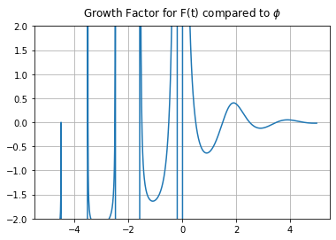
1. Show that \(F(t+1)/F(t) - \phi\) is exactly zero whenever \(t\) is half-way between integers, and is maximum not when \(t\) is an integer but a fixed amount (with a somewhat strange exact expression, namely \(-\arctan((2/\pi)\ln\phi)/\pi\)) less than an integer.
This activity is plain algebra and calculus to start. We did this with a computer algebra system; manipulation by hand is a bit tedious, and at this level there is no advantage to hand computation. To see that it’s true without calculus, a plot works. But this is not a proof, although pretty convincing. One advantage of a plot over a “proof” is that you can see that there are extra features for negative \(t\), namely singularities when \(F(t) = 0\). Indeed this helps to motivate the next activity.
def F(t):
    phi = (1+np.sqrt(5.0))/2
    return((phi**t - np.cos(np.pi*t)*phi**(-t))/np.sqrt(5.0))

t = np.arange(-5,5,0.01)  # Make a fine grid of t values
phi = (1+np.sqrt(5.0))/2
y = [F(tau+1)/F(tau)-phi for tau in t]
fig, ax = plt.subplots() # Cartesian is default, anyway
ax.plot(t, y)
ax.grid(True) # show intersections
plt.ylim(-2,2)
ax.set_title("Growth Factor for F(t) compared to $\phi$", va='bottom')
plt.show()
2. Show that \(F(t)\) has an infinite number of real zeros, and these rapidly approach negative half integers as \(t\) goes to \(-\infty\).
Since the negative Fibonacci numbers \(F_{-k} = (-1)^{k-1}F_k\) alternate in sign, by the intermediate value theorem there must be a zero between \(F(-1)=1\) and \(F(-2)=-1\), another between \(F(-2)=-1\) and \(F(-3)=2\), and so on. That establishes the first part. To do the second, use Binet’s formula and notice that \(\phi^t\) gets very small for large negative \(t\). This forces the zeros to be very nearly the same as the zeros of \(\cos\pi t\), which occur at half-integers. You can use Newton’s method to get the asymptotic formula
This formula already gives for \(k=1\) the answer \(-1.575\), where the true zero is approximately \(-1.570\). The agreement only gets better for larger \(k\). By \(k=5\) the formula gives more than five decimals accurately; by \(k=14\) it gives full double precision accuracy. Since \(\phi = 1.618\ldots\) is bigger than \(1\), in the limit as \(k \to \infty\) the zeros approach half-integers.
3. Rearrange the Fibonacci recurrence relation to
and by making an analogy to finite differences argue that the golden ratio \(\phi\) “ought to” be close to \(\exp(1/2)\). Show that this is in fact true, to within about \(2\) percent.
The central difference on the left is a (very crude) approximation to \(F'(t)\), the derivative at \(t\). Solving the differential equation \(F'(t) = F(t)/2\) gives \(F(t) = C\exp(t/2)\), which grows by a factor \(\exp(1/2)\) when \(t\) is incremented by \(1\). But Fibonacci numbers grow by a factor \(\phi\) when \(n\) is incremented by \(1\). So \(\exp(1/2) = 1.648\ldots\) ought to be close to \(\phi = 1.618\ldots\). And, it is! We found this fact very surprising, and there may be something deeper going on.
4. Draw a phase portrait showing the complex zeros of \(F(t)\). Give an approximate formula (asymptotically correct as \(\Re(t)\) goes to plus infinity) for the locations of these zeros.
This activity is connected with a (quite new) development in the presentation of complex functions, namely the use of phase portraits, as done at the link above. This was first used (to our knowledge, anyway) by Elias Wegert in his book Visual Complex Functions but has since been used to very great effect. It turns out that one can, after all, make a useful two-dimensional plot of a complex function, by plotting the argument of \(F(z)\) in colour according to a colour wheel given by the simple plot of the function \(F(z) = z\). If your software plots the real axis for that simple function as (say) light blue, then the line of light blue in your plot of the more complicated \(F(z)\) tells you what \(F\) does to the real axis. Similarly for the sectors. One key point is that zero (for the simple function \(F(z)=z\)) has all colours touching it and moreover if you circle around zero clockwise you get a particular sequence of colours (say, blue, green, yellow, red) by the time you get back to where you started. If you see a point in the phase portrait of your complicated function \(F(z)\) which has all colours, in that order clockwise, then you have located a place where \(F(z)=0\). You can see the zeros of a complex function on the graph!
You can also see poles, because the colours will be the same but go clockwise instead. Branch cuts and other things are also visible.
It takes a bit of getting used to, but surprisingly little. And, besides, the pictures are very pretty.
To find approximate locations of the zeros, set \(F(t) = 0\). This gives the equation
using the complex expression for cosine. We now put \(t = \sigma + i\tau\) and explore what happens when both \(\sigma\) and \(\tau\) are large and positive (a similar thing can be done in the lower half plane). By comparing the magnitudes of the left and right hand side, and neglecting the term in the cosine that is small (being multiplied by \(\exp(-\pi\tau)\)) we get the following approximation:
If we plot this line we see a pretty good match with the line of zeros.
By comparing the arguments we get a similar-looking equation:
where now \(K\) can be any integer. Setting these exponents to be equal, we get a second (linear) equation relating \(\sigma\) and \(\tau\). These two equations can be solved to get the following approximate locations for the zeros.
We show four choices of \(K\) (it turns out we need negative integers \(K\)) in the following figure. The agreement is pretty good even for the smallest magnitude zero, and it only gets better as we compare larger zeros.
Since the zeros come in conjugate pairs, if \((\sigma,\tau)\) is a zero then so is \((\sigma,-\tau)\).
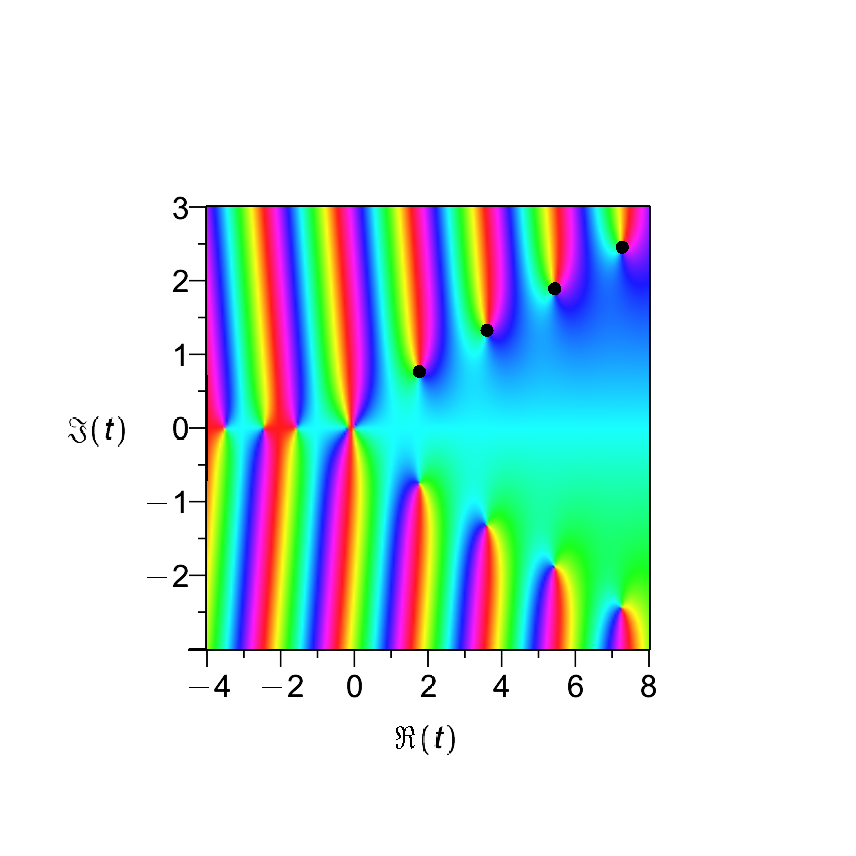
Fig. 13 This phase portrait shows the zeros of the continuous Fibonacci function. The black dots on the top right are from the approximate formula.#
5. The angles satisfy \(\cos \theta_n = F_n/(2F_{n-1})\), and these rapidly tend to \(\pi/5\) with cosine \(\phi/2\). So the cumulative sum to, say, \(N\) terms is going to approach
and the detailed behaviour of the \(\cdots\) is going to be of interest. We find (this is an unverified solution, unpublished elsewhere) that
and we have numerically found that \(c_0 \approx -0.565677757047407\) and \(c_2 \approx 1.37638192047117\). We’d actually like to know more about this.
Fibonacci Activity 15: Truncated Power Series#
We want you to program the algebraic operations for Truncated Power Series (TPS for short).
We describe a very basic implementation of Truncated Power Series in Python. We are not going to use anything fancy (such as operator overloading, or object-oriented programming) although using those would really make the package easier to use and understand. The purpose of this is not use per se, but rather practice in programming. And we are just beginning, here. So we take it slow.
The first thing is to decide what data structure to use. We choose a simple list as our basic data structure: a Truncated Power Series will be represented by a list of its coefficients. To keep things simple, we make all our lists have the same length, which we will call Order (like the Maple variable for its series command).
Order = 8
# This series is 0 + 1*x + 0*x^2 + ... + 0*x^{Order-1} + O(x^Order)
x = [0, 1]
for i in range(2,Order):
    x.append(0)
print(x)
[0, 1, 0, 0, 0, 0, 0, 0]
geom = [1 for i in range(Order)]
print(geom)
[1, 1, 1, 1, 1, 1, 1, 1]
def addTPS(a, b):
    c = []
    for i in range(Order):
        c.append(a[i] + b[i])
    return(c)
def scalarMultiplyTPS(alpha, a):
    c = []
    for i in range(Order):
        c.append(alpha*a[i])
    return(c)
print(scalarMultiplyTPS(13, geom))
print(addTPS(x, geom))
[13, 13, 13, 13, 13, 13, 13, 13]
[1, 2, 1, 1, 1, 1, 1, 1]
def multiplyTPS(a, b):
    c = []
    for i in range(Order):
        tmp = 0
        for j in range(i+1):  # Why is it i+1 here and not "i" ? (Rhetorical question)
            tmp += a[j]*b[i-j]
        c.append(tmp)
    return(c)
print(addTPS(geom, geom))
[2, 2, 2, 2, 2, 2, 2, 2]
oneminusx = [1,-1]
for i in range(2,Order):
    oneminusx.append(0)
print(oneminusx)
print(multiplyTPS(oneminusx, geom))
[1, -1, 0, 0, 0, 0, 0, 0]
[1, 0, 0, 0, 0, 0, 0, 0]
This represents the “well-known” geometric series fact that
print(multiplyTPS(geom, geom))
[1, 2, 3, 4, 5, 6, 7, 8]
We can understand this if we know that the derivative of \(1/(1-x)\) is \(1/(1-x)^2\) and the derivative of the geometric series is \(0 + 1 + 2x + 3x^2 + 4x^3 + \cdots\). If we don’t know any calculus, we can multiply the TPS out by hand to see that it’s true.
def divideTPS(a, b):
    d = [a[0]/b[0]] # Will divide by zero if b[0]=0
    for i in range(1,Order):
        tmp = 0
        for j in range(1,i+1):
            tmp += b[j]*d[i-j]
        d.append((a[i]-tmp)/b[0])
    return(d)
one = [1]
for i in range(1,Order):
    one.append(0)
newgeom = divideTPS(one, oneminusx)
print(newgeom)
[1.0, 1.0, 1.0, 1.0, 1.0, 1.0, 1.0, 1.0]
The use of / in the procedure divideTPS meant that the results were automatically floating point numbers.
print(divideTPS(newgeom, geom))
[1.0, 0.0, 0.0, 0.0, 0.0, 0.0, 0.0, 0.0]
phipoly = [1, -1, -1 ]
for i in range(3,Order):
    phipoly.append(0)
print(phipoly)
FibonacciGenerator = divideTPS(x, phipoly)
print(FibonacciGenerator)
[1, -1, -1, 0, 0, 0, 0, 0]
[0.0, 1.0, 1.0, 2.0, 3.0, 5.0, 8.0, 13.0]
def raisePowerTPS(a, alpha):
    # We implement the JCP Miller recurrence relation to compute a**alpha
    a0 = a[0]
    if a0==0:
        raise ValueError( "Leading coefficient shouldn't be zero")
    y = scalarMultiplyTPS(1/a0, a) # Has leading coefficient 1
    c = [1]
    for i in range(1,Order):
        tmp = 0
        for j in range(i):
            tmp += (alpha*(i-j)-j)*c[j]*y[i-j]
        c.append( tmp/i )
    return(scalarMultiplyTPS(a0**alpha, c))
square = raisePowerTPS(geom, 2)
print(square)
[1, 2.0, 3.0, 4.0, 5.0, 6.0, 7.0, 8.0]
half = raisePowerTPS(square, 0.5)
print(half)
[1.0, 1.0, 1.0, 1.0, 1.0, 1.0, 1.0, 1.0]
# bad = raisePowerTPS(x, 2) # Test of error message (leading coeff of "x" is zero)
Here’s the error message that occurs when that last cell is uncommented (remove the # from the start of the line)
ValueError                                Traceback (most recent call last)
Input In [66], in <module>
----> 1 bad = raisepowerTPS( x, 2 )

Input In [63], in raisepowerTPS(a, alpha)
      3 a0 = a[0]
      4 if a0==0:
----> 5     raise ValueError( "Leading coefficient shouldn't be zero")
      6 y = scalarMultiplyTPS( 1/a0, a ) # Has leading coefficient 1
      7 c = [1]

ValueError: Leading coefficient shouldn't be zero